It may not be practical to automatically create a graph for a problem
in order to search it.
This presentation describes an alternative to graph search,
called
state space search, that can solve problems without
graphs.
Here is a typical 8-puzzle problem:
The current state is just one of a number of possible configurations of
the 8-puzzle.
Regarding the blank as one of the tile positions, there are 9!
=
362,880 possible configurations.
- It can be proven that only half of these
are reachable from a given state.
- So the number of states that are reachable from the current
state is 181,440, including the goal state.
Our graph creation algorithm can create and connect 181,440 8-puzzle
states in a reasonable amount of time.
Consider a typical
15-puzzle problem:
| Current State |
Goal State |
| 7 |
14 |
|
9 |
| 10 |
2 |
11 |
13 |
| 6 |
15 |
4 |
12 |
| 5 |
1 |
8 |
3 |
|
| 1 |
2 |
3 |
4 |
| 5 |
6 |
7 |
8 |
| 9 |
10 |
11 |
12 |
| 13 |
14 |
15 |
|
|
A graph for the 15-puzzle would have 16!/2 =
10,461,394,944,000
vertices — far too many to create and connect in a graph.
We define a
state space for a problem as the set of states
reachable from the problem's current state using the problem's moves.
A state space is an
abstraction, while a problem graph is
a
concrete data structure. Our graph creation algorithm actually
creates the entire state space for a problem.
We will describe an algorithm that:
- Does not require a problem graph made in advance,
- Traverses just enough of a problem's state space to
solve it, that is, to find a path from the current state to the
goal state, and
- Creates a predecessor tree, like that produced by the graph
search algorithm, that can be used to present a solution.
Then we will implement the algorithm as an
abstract class
that can be extended to create specific kinds of problem solvers,
including one that does use a problem graph, and others that do not.
Recall the breadth-first graph search algorithm at right, with the
parameter
s representing the start vertex
The parts indicated in
red show the
dependence of the algorithm on the pre-existence of a graph
G
with:
- Vertices given an initial open status that is used to test
whether they are reencountered in the search, and
- An adjacency list representation
We will rewrite the algorithm so that the dependence on
G
is removed.
BFS(G,s)
   for each u ∈ V[G]-{s} do
      open[u] = true
      d[u] = ∞
      pred[u] = null
   open[s] = false
   d[s] = 0
   pred[s] = null
   Q = {s}
   while Q ≠ {} do
      u = Remove[Q]
      for each v ∈ Adj[u] do
         if open[v] = true
            then open[v] = false
                 d[v] = d[u] + 1
                 pred[v] = u
                 Add(Q,v)
First, we specify an abstract
expand operation that replaces the
use of a graph's adjacency list.
expand takes a vertex
u representing a problem state
s as
an argument and returns all the vertices representing states that are
one move away from
s.
- If a graph for the problem exists, expand(u) can be
defined to return the same thing as Adj[u].
- If a graph does not exist, expand(u) can be
defined to dynamically create the possible next states and return
them as new vertices.
At right we have replaced
Adj[u] with
expand(u) (in
blue). We have also renamed the
algorithm as
Search and removed the parameter
G.
Search(s)
   for each u ∈ V[G]-{s} do
      open[u] = true
      d[u] = ∞
      pred[u] = null
   open[s] = false
   d[s] = 0
   pred[s] = null
   Q = {s}
   while Q ≠ {} do
      u = Remove[Q]
      for each v ∈ expand(u) do
         if open[v] = true
            then open[v] = false
                 d[v] = d[u] + 1
                 pred[v] = u
                 Add(Q,v)
The graph search algorithm uses a vertex's
open status to
determine if it has already been encountered in the search. If it has
been encountered it is ignored.
We can accomplish the same thing without having the vertices created in
advance:
- Maintain a set V of vertices that have already been seen
in the search
- If a vertex v in expand(u) is in V, ignore
it
- Otherwise, add v to V and process it just like the
graph search algorithm
The algorithm is shown at right with new modifications
in
blue.
Search(s)
   d[s] = 0
   pred[s] = null
   Q = {s}
   V = {s}
   while Q ≠ {} do
      u = Remove[Q]
      for each v ∈ expand(u) do
         if v ∉ V
            then put v in V
                 d[v] = d[u] + 1
                 pred[v] = u
                 Add(Q,v)
Rather than traverse an entire state space for a problem, like a
breadth-first graph search,
Search will stop when it encounters
a vertex representing the problem's final state:
- We specify a boolean success operation that takes a vertex
as argument and returns whether it represents a final state
- Each time the algorithm removes a vertex u
from the queue, if success(u) is true the algorithm stops
and u is returned
- If the queue is emptied and no final state has been encountered,
the algorithm stops and null is returned
The final algorithm is shown at right with new modifications
in
blue.
Search(s)
   d[s] = 0
   pred[s] = null
   Q = {s}
   V = {s}
   while Q ≠ {} do
      u = Remove[Q]
      if success(u)
         then return u
      for each v ∈ expand(u) do
         if v ∉ V
            then put v in V
                 d[v] = d[u] + 1
                 pred[v] = u
                 Add(Q,v)
   return null
This section presents an abstract class
Solver that supports
automatic problem solving.
Solver will be the superclass of various concrete subclasses
that implement different kinds of search.
To compare the performance of these searches it is useful to compile
search statistics, so we first describe a
Statistics class for this
purpose.
Solver and
Statistics will join
SolvingAssistant
in the
framework.solution package.
The efficiency of state space search can be quantified by keeping track
of the statistics described below.
Each statistic description is followed in parentheses by the string
constant used as a key to refer to the statistic in Java code.
- The number of vertices created (VERTICES)
- The length, that is, the number of moves in a solution, if one is
found (LENGTH)
- The time, in milliseconds, taken to complete the search
(TIME)
- The number of queue operations (adds and removes) during the
search (NUM_OPS)
- The maximum size of the queue during the search
(QUEUE_SIZE)
- The number of times a vertex is reencountered, that is, a
solution path "circularity" is ignored, during the search
(CIRCULARITIES)
The
Statistics class has a constructor with no arguments that
creates an object with fields for each of the search statistics
initialized to zero.
The
setHeader method accepts a string header to be used
when the object is displayed.
The
toString method is overridden so
that the following code produces the output below.
Statistics Example
------------------------------
Vertices created   0
Solution length   0
Solution time   0
Num of queue ops   0
Max queue size   0
Circularities   0
A
Statistics object can be further manipulated by using the
methods below. Each method requires a string
key naming the
particular statistic involved.
- getStat(key): returns the value of the statistic named
by key as an integer
- putStat(key, value): sets the value of the statistic named
by key to the integer value
- incrStat(key): increments the value of the statistic named
by key by one
Here is an example of their use on the
TIME statistic,
with the result shown below:
Statistics Example
------------------------------
Vertices created   0
Solution length   0
Solution time   314160
Num of queue ops   0
Max queue size   0
Circularities   0
Here are representative statistics for breadth-first and depth-first
search for the 5-move 8-puzzle problem:
Breadth-First State Space Search
------------------------------
Vertices created   87
Solution length   5
Solution time   3
Num of queue ops   138
Max queue size   37
Circularities   50
|
Depth-First State Space Search
------------------------------
Vertices created   181432
Solution length   147
Solution time   1258
Num of queue ops   362727
Max queue size   48728
Circularities   302041
|
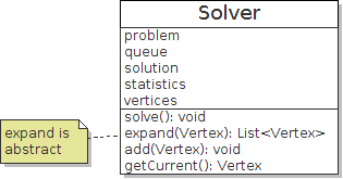
The search algorithm will be implemented in an abstract
Solver
class.
A
Solver object stores references to these previously discussed
class objects:
- The Problem to be solved
- The Queue used to control the search
- The Solution obtained if one is found
- The Statistics computed during the search
- The HashMap used to store vertices during the search
The
Solver API includes:
- Various getters and setters for the stored
objects
- A solve method that attempts to solve the problem from its
current state, producing statistics and a solution if possible
- An abstract expand method used by the search algorithm that must
be provided by a subclass
- An add method used by the search algorithm to add vertices to the
queue, which may be overridden by subclasses for various kinds of
search
- A getCurrent method used by the search algorithm to get the
starting state as a vertex, and which may be overridden by
subclasses
A UML class icon for
Solver is shown below.
A listing of
Solver.java is available from the menu. Note that
the
search method must be provided by students.
Solver.java should be added to the
framework.solution
package.
An application using the abstract
Solver class provides a
subclass that:
- Must implement the expand method, and
- May change the type of queue used for searching
This section describes four subclasses of
Solver:
- GraphSolver: for breadth-first and depth-first search of
problems with graphs already created
- StateSpaceSolver: for breadth-first and depth-first search of
problems without graphs
- BestFirstSolver: for non-optimal heuristic search using a
priority queue
- AStarSolver: for optimal heuristic search using
the A* algorithm