Station Builder V1.2
Transportation Data Research Lab
NATSRL, UMD
Station Builder is a tool developed for analyzing daily traffic at the station level, where a station is defined as a set of detectors located in a close proximity. This is an initial version developed for visualization of traffic flow and occupancy through various means, but future versions will include tools that would allow analysis for more advanced parameters such as congestion indexes and speed variability measurements. In station data, station volume is the total number of vehicles counted from the detectors that belong to that station within the measurement period. The computation of station occupancy can have many variations. In this software, station occupancy can be generated using two methods: (1) arithmetic average and (2) worst case. Arithmetic average is computed by dividing summation of occupancies of the detectors by the number of detectors. Worst case is computed by choosing the maximum occupancy among the detector occupancy. It is believed that worst-case computation of occupancy is considered a better representation, if you are analyzing traffic congestion using station occupancy.
The main features of this version include:
- Volume color grid plot of any road in any time range.
- Occupancy color grid plot of any road in any time range.
- Occ contour plot of any road in any time range.
- Vol/occ scater plot for any station in any time range
- Vol/Occ line graph for any station in any time range
- Allows export to Excel data format.
- You can easily define your own stations using simple text editing.
- You can easily define your own road segments using simple text editing.
- Many 3-D rendering and graphics editing capability.
- You can see all of the *.traffic file compression rate and file list in one table.
A sample station definition file is copied to the installation directory upon installation, which includes 866 stations defined by the Traffic Management Center of Mn/DOT. You can find this file from the installation directory.
If you have successfully installed this software, you would be able to see the initial screen given below.
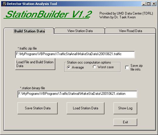
The first step required is building (or computing) a station data from a *.traffic file (detector data) using the Build Station Data button. Before you clicking this button, you should choose one of the occupancy options you have: (1) average and (2) worst case. If a lane shows a volume or occupancy hardware error, such as negative values, (it means that that particular detector is not functioning correctly), the occupancy for that malfunction detector is excluded from the station occupancy computation for either option.
If you check mark on the “Save zip file info” check button, the software produces the zip compression information of the *.traffic file you selected, and store the information in a text file named “zipFileInfo.txt” in the installation directory. A slice of this file information is shown below:
Number of files in zip file: 7430
Zip index, Compressed Size, Extract Size, file name
0 780 5760 2.o30
1 389 2880 2.v30
2 250 5760 3.o30
3 140 2880 3.v30
4 22 5760 4.o30
5 20 2880 4.v30
6 592 5760 5.o30
7 306 2880 5.v30
8 765 5760 7.o30
9 366 2880 7.v30
10 2579 5760 8.o30
11 1268 2880 8.v30
12 3163 5760 9.o30
13 1415 2880 9.v30
This file is very useful when you wish to confirm whether a detector file actually exists in the zip file or not. It also gives ideas on how much the data is dense, which gives some inference of how good the detector data is.
Next, I will walk you through how to use the Station Builder, step by step. However, it is important to note that other alternatives and variations exist on how to use this software. It is simply provided as a tutorial.
Step 1: Click on the Load File and Build Station Data button.
This button allows you to generate the station data based on the occupancy computation options you selected. One requirement you must remember is that the Station and Road definition files must exist in the installation directory, i.e. the directory that has the file StationBuilder.ext. The names of the definition files required are:
TMCRoad2Sta.List
TMCSta2Det.List
Above are text files that include a list of detector IDs of stations and a list of stations per road. It is editable using any text editor such as a notepad. In fact, you can add your own definitions of the roads and stations if you wish to redefine or extend the particular section of the road.
Clicking the Load File and Build Station Data button will open a file dialog and lead you to select a *.traffic file as shown below. The screen samples are based on Win 2000.
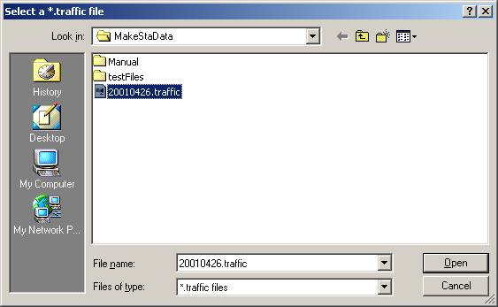
Select the desired file and click the open button. Then the software will start building the station data and will show its progress using a progress bar. The station data building process includes unzipping of nearly 8,000 files and computing 866 stations, so it will take some time depending on your computer speed (typically 10 to 15 seconds) and the number of stations defined in the station definition file.
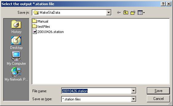
Step 2: Click on the Save Station Data button
(optional)
After creating the station data in Step 1, you can save the created station data in a binary form and reuse it later without the need for re-computing and recreating the station data. It will save you time. Directly loading the station is significantly faster than loading the detector data *.traffic file. This pre-computed station data file has a file extension “*.station,” which the software will suggest to the user through a file dialog when you click on the Save Station Data Button. Go ahead and use the default name as suggested by the software. The example is shown below.
Next time when you load the data, you should simply load this saved data using the Load the Station Data button.
Step 3: Click on the View Station Data tab
From this tab, you will be able to view and plot all of the stations defined in the TMCSta2Det.List file. This tab is used for a single station analysis.
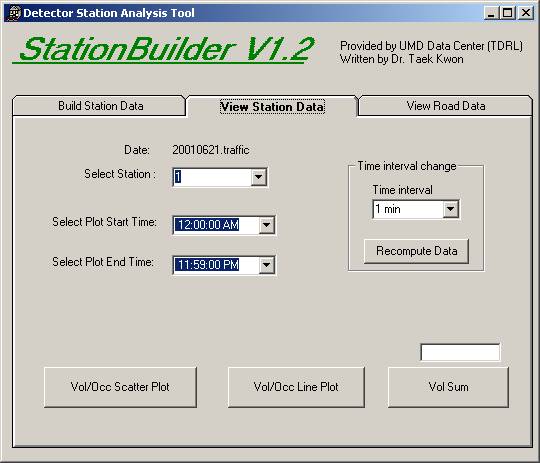
Step 4: Select the Time interval combo button and
click on the Reompute button.
The default time interval loaded is the 30sec data. If you wish to see the data in other time interval, select one of the Time interval combo button and click on the Recompute button. It will create new data with a new time interval and will change the time intervals available in the Start and End time combo buttons. Station Builder provides time interval choices of 30sec, 1min, 2min, 3min, 4min, 5min, 10min, 15min, 30min, and 1hour.
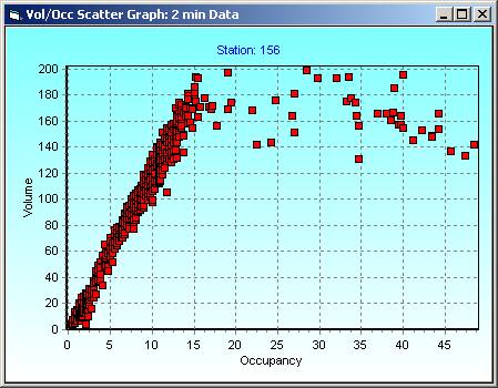
Step 5: Click on the Vol/Occ Scatter Plot button
It shows vol/occ relation of the selected station using a standard scatter plot. A sample is shown below. You can also edit the graph or see the data by clicking on the left axis. Please make sure to select the Plot End Time bigger than Plot Start Time; otherwise, Station Builder will complain.
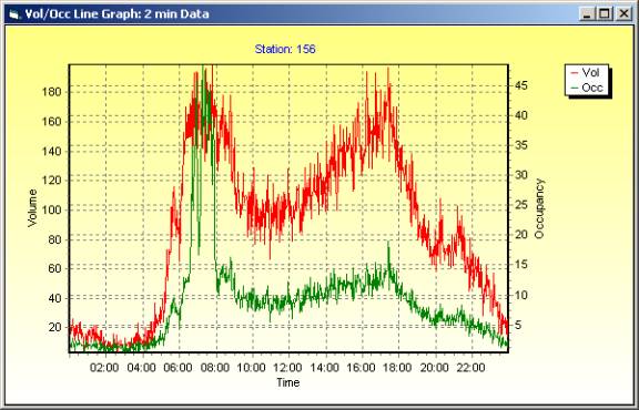
Step 6: Click on the Vol/Occ Line Plot button
It shows the vol/occ relation using two lines as shown below. You can zoom in the graph by dragging mouse with left button down or recover from the zooming by dragging in the reverse direction. Again, clicking on the left axis gives you the graph editing and manipulation tools.
Step 7: Click on the Vol Sum button.
It computes the total volume of the selected time range of the station, in the text box just above the Vol Sum button. It gives a simple way of knowing how many vehicles were present during the time span between the Plot Start Time and Plot End Time for the selected station. It will be useful if you wish to know, for example, daily traffic.
Step 8: Click on the View Road Data tab
This tab is mainly used for the road level analysis. One important note is that this tab uses the time range and intervals defined in the View Station Data tab, so make sure to select the time ranges and the interval from the View Station Data tab.
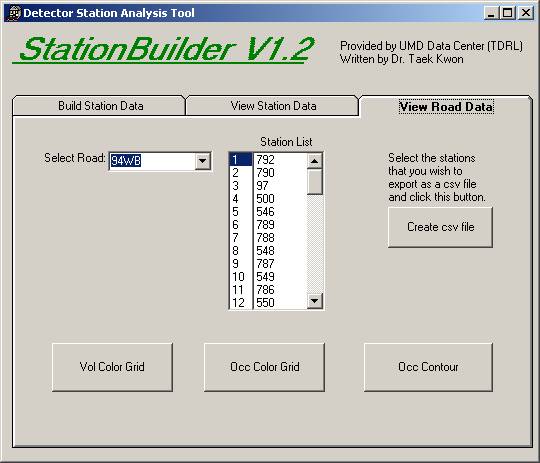
When you select a road, you will see the station list of the selected road from the table in the middle. It is ordered according to the direction of traffic flow, i.e. from upstream to down stream.
Step 9: Select a road from the Select Road combo
box
Select a road from the list available from the Select Road combo box. The list is loaded from the “TMCRoad2Sta.List” file.
Step 10: Click on the Vol Color Grid button.
The volume of the road for the time range selected is plotted using a color grid map. The red color indicates high volume while the green color indicates a low volume. A plot example is shown below.
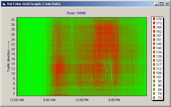
Step 11: Click on the Occ Color Grid button.
The occupancy of the road for the time range selected is plotted using a color grid map. The red color indicates high occupancy, while the green color indicates a low occupancy.
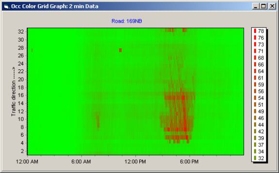
One interesting state you want to observe is that high volume does not mean that there is congestion. The two graphs shown above clearly demonstrate that effect. Note from the volume color grid that traffic volumes were heavy in both morning and afternoon. However, note from the occupancy color grid that there was no congestion in the morning, but had congestion in the afternoon. Therefore, it is always important to look at both the volume and occupancy grids side by side for your analysis. Volume will tell you only the half of the story. You can also observe traffic shockwave effect from the occupancy color grid between 2:00pm and 6:00pm, in which downstream traffic is gradually backed up to the upstream with stop and go state. It indicates that there were high variances in the speed in that period. According to FHWA recommendations, low speed variance should be considered the more urgent goal of traffic control than reducing the total travel time.
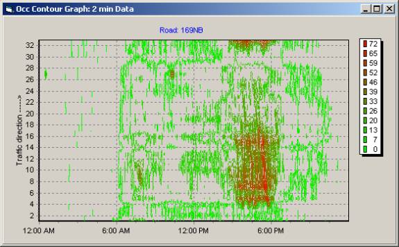
Step 12: Click on the Occ Contour button
It shows a similar traffic effect as the occupancy color grid except that it shows the occupancy as a contour plot. Similar types of analysis as the occupancy color grid can be made using this graph. A sample plot is shown below.
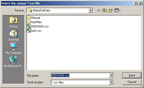
Step 13: Exporting station data into an Excel readable file.
Station builder includes a function that allows exporting the station data into a Microsoft Excel readable spreadsheet file. First, select the stations using the Station List list-box in the View Road Data tab. You can use the Shift key with mouse click or Control key with mouse clicks to select multiple stations. Similarly to all other cases, the time range should be selected using the View Station Data tab. If all the required selections are ready, then just click on the Create csv file button. Station Builder will open a file dialog box and suggest a filename. Accept the default name or type in a file name without the extension, then click on the Save button. The saved file now can be loaded to Excel for further analysis or data processing. Since the output file is a comma separated file, it can be easily imported to other data analysis as well.
Provided by,
Dr. Taek M. Kwon, Professor
Transportation Data Research Lab,
A Part of Northland Advanced Transportation Systems Research Lab
University of Minnesota Duluth