Part 2: Populations and Phylogenetics

Basics of trees as graphs

Phylogenetic and other trees in bioinformatics are usually considered as graphs. We will describe some fundamental definitions of graphs that are relevant to our study of trees.

A graph is a set of vertices, $V$ , along with a set of edges $E$ . An edge is a pair of vertices. If two vertices are in a edge, we say they are adjacent, and if an edge contains a vertex we say the vertex is incident to the edge.

The degree of a vertex is the number of edges to which it is incident.

A graph isomorphism is a bijection G sending a vertex set of one graph, V to that of another, V', with e in E equivalent to e' in E' where e' is the image of vertices in e.

Trees are connected, acyclic graphs (i.e. there are no loops of edges). This is equivalent to being a connected graph with $|V|-1$ edges; it is also equivalent to there being a unique path betweeen any two vertices.

In a tree, vertices with only one edge are called leaves; others are interior vertices. An edge incident to a leaf is a pendant edge, otherwise it is an interior edge.

The star tree is an important type of tree which has a single interior vertex. If a tree is not a star, then it has two interior vertices which are each adjacent to exactly one nonleaf vertex.

A caterpillar is a tree in which all of the interior vertices are on a single path.

A rooted tree has a unique interior vertex labeled as the root, and the edges are considered directed away from the root towards the leaves.

The automorphism group of a tree is the group of graph isomorphisms sending a tree to itself; for rooted trees, these are determined by the action on the leaves (their least common ancestors must match up).

The median of three vertices in a tree is the unique intersection of the three paths between the vertices.

A centroid of a tree is a vertex that produces the smallest maximum vertex subtree after being deleted. A theorem of Jordan (1869) is that every tree has one or two centroids (if they two must be adjacent).

A center of a tree is a vertex minimizing the distance from it to any other vertex. As for centroids, there are either 1 or 2 centers of any tree.

Phylogenetics

Phylogenetics is the study of evolutionary relationships inferred from genetic data. The goal is to reconstruct the correct evolutionary tree.

In describing an evolutionary tree, there is a fundamental distinction between rooted and unrooted trees. A rooted tree has a special node, the root, which is the ancestor of all other nodes in the tree. Sometimes the goal of a phylogenetic analysis is to determine the root; for example in epidemiological settings, it is useful to know the root of a novel viral outbreak. However most methods of phylogenetics produce an unrooted tree, in which the root is undetermined. This can be partially worked around by including in the analysis some data from an outgroup - something which is known to be more evolutionary distant from all of the other entities in the dataset. For example, if the goal is to construct a phylogeny of mammals, we could choose to include sequence data from outside the mammals such as a frog, reptile, or bird.

A bifurcating, or binary tree has exactly three edges from each interior node; another way to say this is that each interior node has degree three.

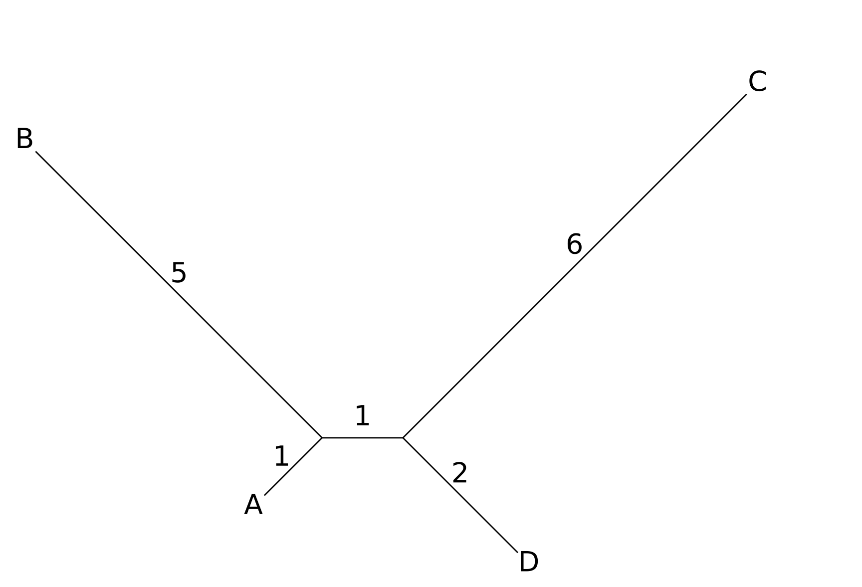
Trees are often described using the Newick format (named after a restaurant in Dover, New Hampshire, where the format was developed over dinner). As an example, the unrooted tree below:

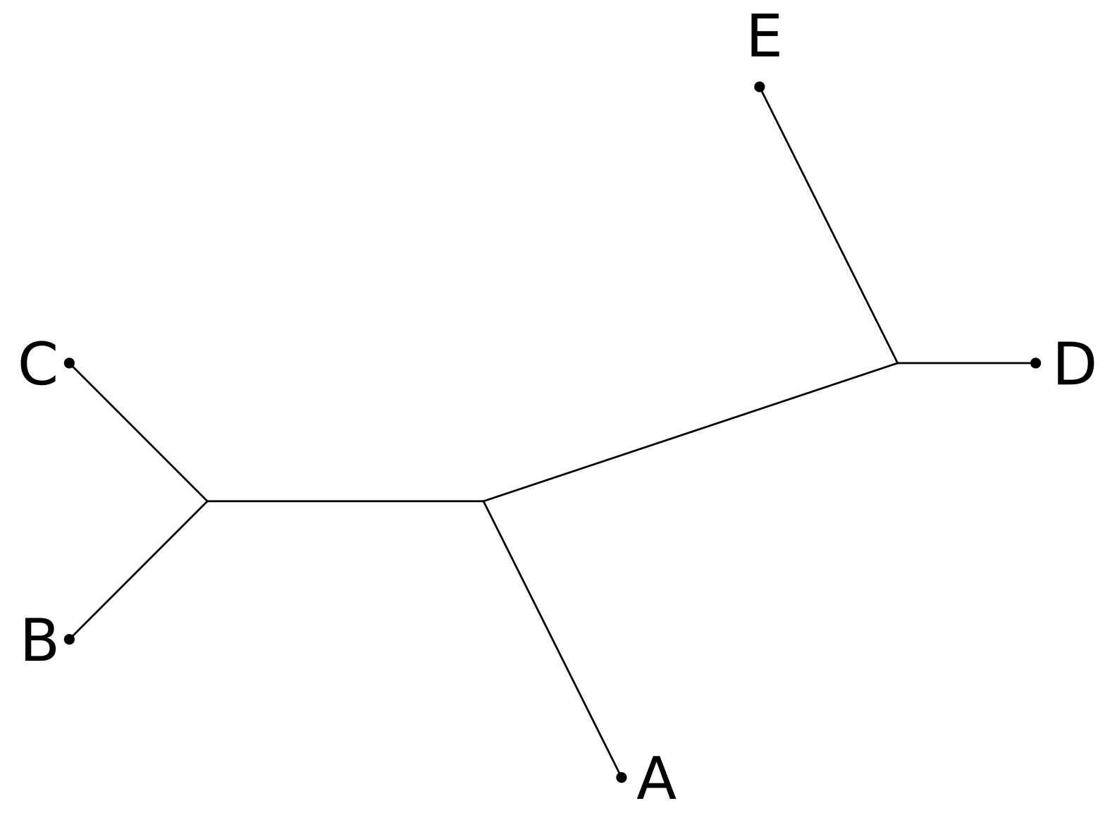
could be represented in Newick format as $$(((B: 1.4, C:1.4) : 2, A : 2.24): 3.16, D: 1, E: 2.24) $$ the numbers giving the length of the edges. There is an implicit root node in the Newick format, which means that unrooted trees do not have a unique representation.

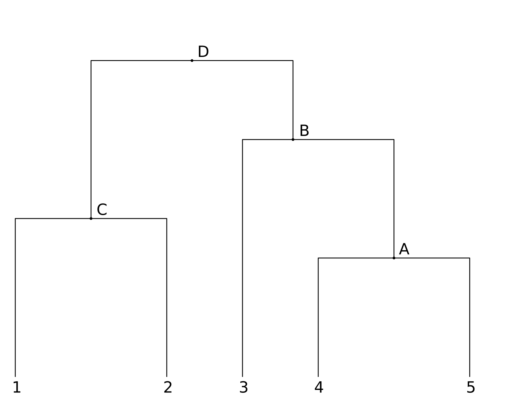
A large forest of trees

It is often useful to think of a phylogenetic problem in two phases: finding the correct tree topology, and then determining the length of each branch in the tree. In problems involving large numbers of taxa the hardest part is the first phase, that of determining the correct topology. This is because of the explosive combinatorial growth in the numbers of possible trees, which we will briefly survey below.

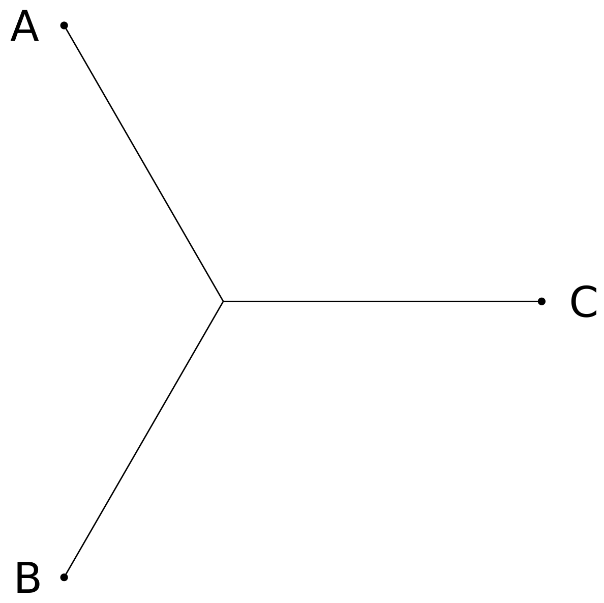
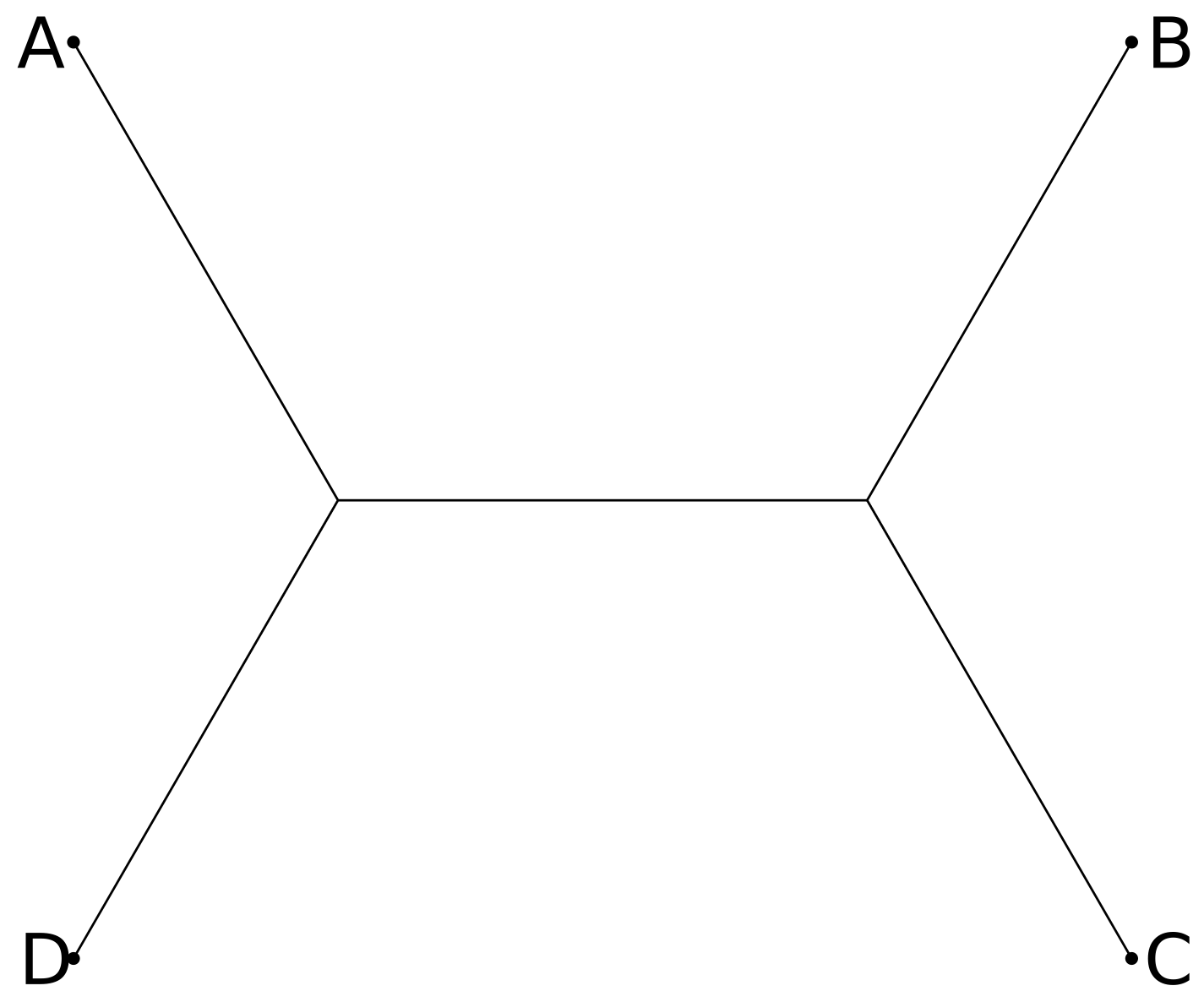
Let us consider the number of topologies of unrooted bifurcating trees. For three taxa, there is only one possibility:

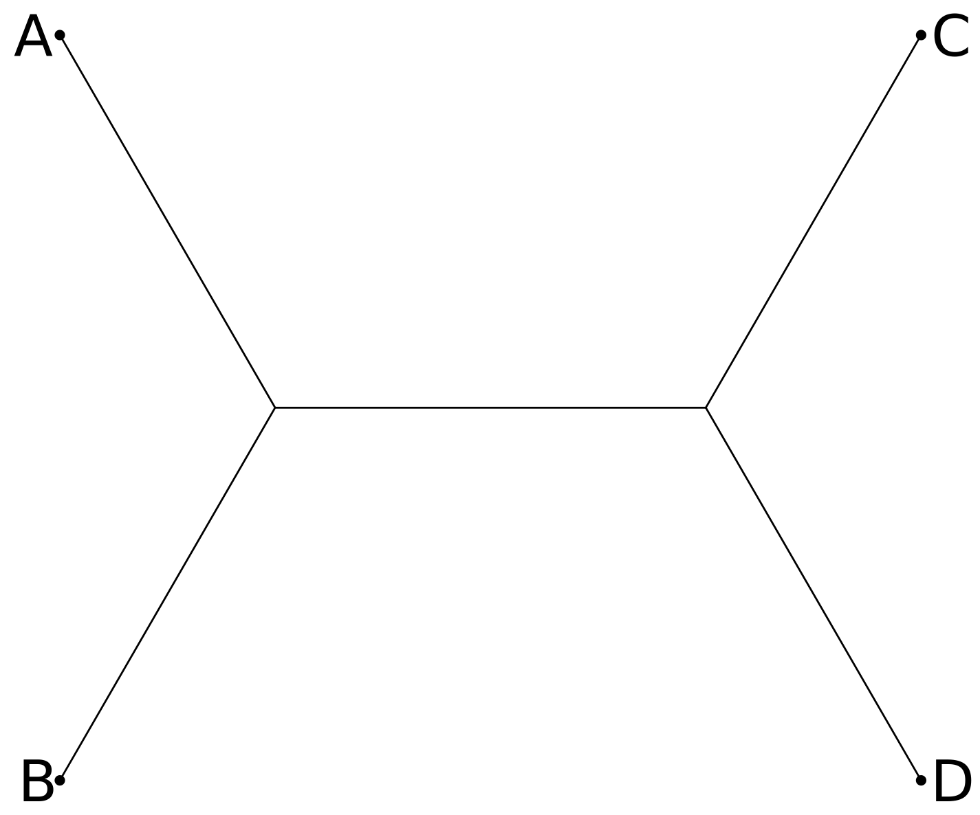
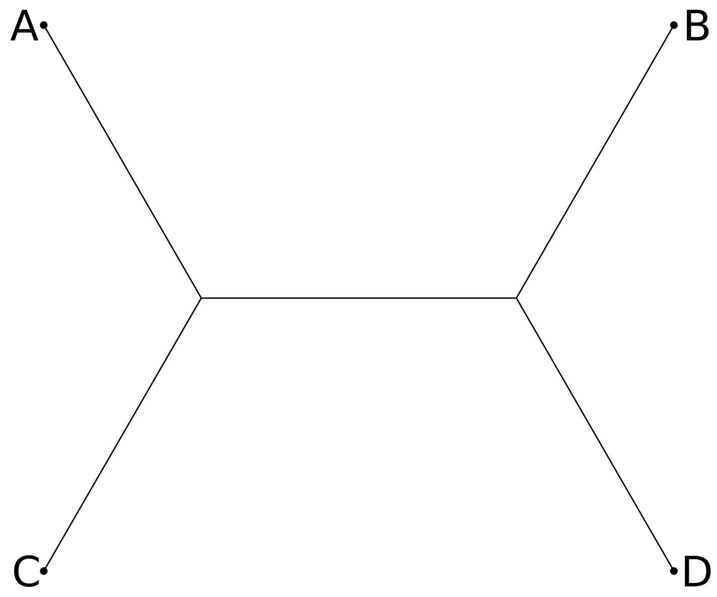
For four taxa $A$ , $B$ , $C$ , and $D$ , we could add a branch with leaf $D$ to any of the three edges of the three-taxa tree of $A$ , $B$ , $C$ , leading to three distinct four-taxa trees:

Continuing with this pattern, we can see that an unrooted tree with $n$ leaves will have $2n-3$ edges, so that if there are $t(n)$ trees with $n$ leaves then $t(n+1) = (2n-3) t(n)$ . Thus

$t(n) = (2n-5)(2n-7)\ldots (3) = \frac{(2n-5)!}{2^{n-3}(n-3)!}.$

The really important aspect of this formula is how quickly it increases with $n$ . For $n=10$ leaves, there are $2,027,025$ unrooted bifurcating trees. For $n=20$ leaves, $t(20) \approx 2.2 \times 10^{20}$ unrooted bifurcating trees. So once we get past about $20$ taxa, it is not feasible to examine every tree.

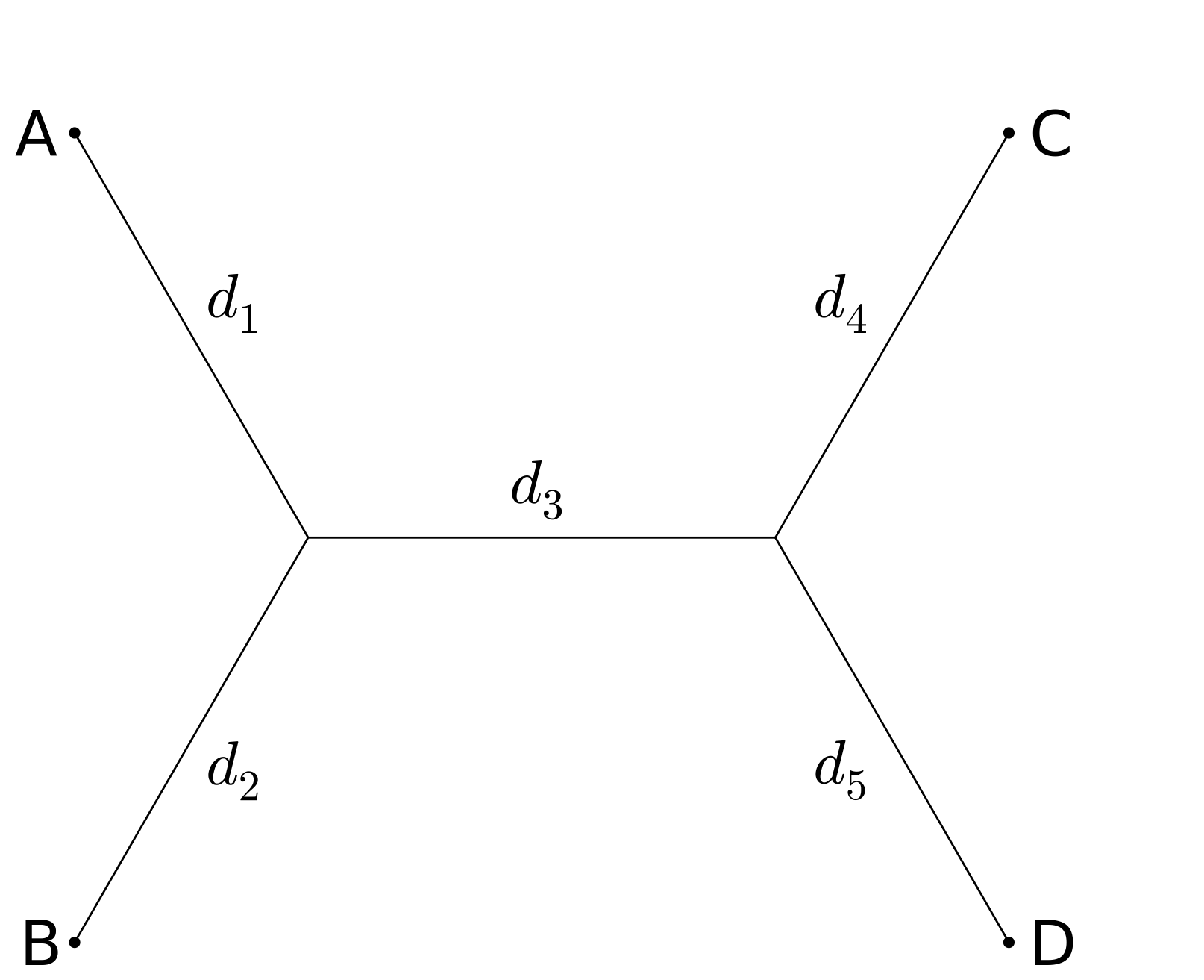
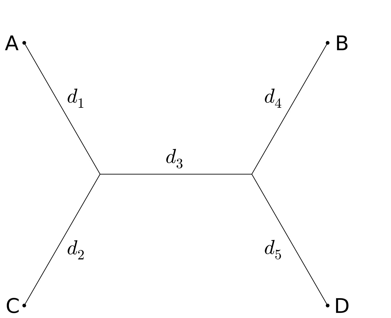
The four-point condition

Since there are only $2n-3$ edges in a bifurcating tree, in general if we are given $n(n+1)/2$ pairwise distances we can cannot find a tree that induces those distances.

A famous result by Peter Buneman (1973) is that a set of pairwise distances between leaves is only compatible with a tree structure if all possible "four-point conditions" are satisfied. The four-point condition for leaves A,B,C, and D is that among the three quantities $d_{A,B} + d_{C,D}$ , $d_{A,C} + d_{B,D}$ , and $d_{A,D} + d_{B,C}$ , two of them must be equal and not less than the third.

Tree Rearrangments

Because the number of tree topologies grows so quickly as we add taxa, it is usually unfeasible to search the entire space for the "best" tree, regardless of what we consider "best". So most phylogeny methods heuristically search through a relatively small portion of the space of tree topologies, hopefully concentrated in regions with trees that fit the data well. In order to move around tree space, we need to have some standard types of moves which rearrange the branches of the tree. There are many choices for these moves; we will just examine two of the more popular and useful tree rearrangements: Nearest Neighbor Interchange (NNI) and Subtree Pruning and Regrafting (SPR).

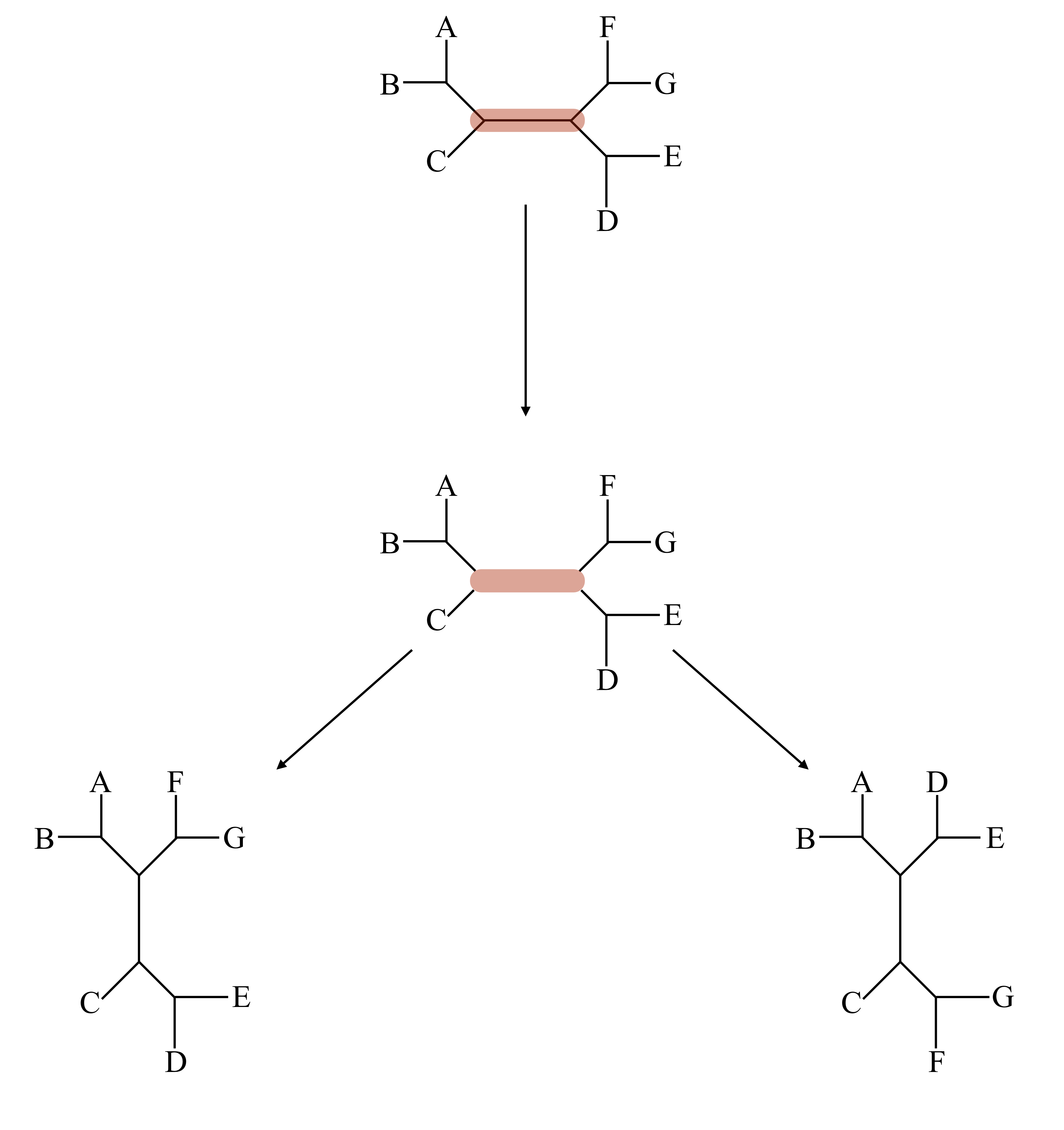
In a NNI move we delete an internal edge in the tree along with its two internal nodes, leaving us with four free internal edges. These edges can be recombined to make a bifurcating tree in three ways: the original way, and two others, as shown below. Since there are $n-3$ internal edges, NNI gives $2n-6$ options for rearrangement of a given tree with $n$ leaves.

NNI example

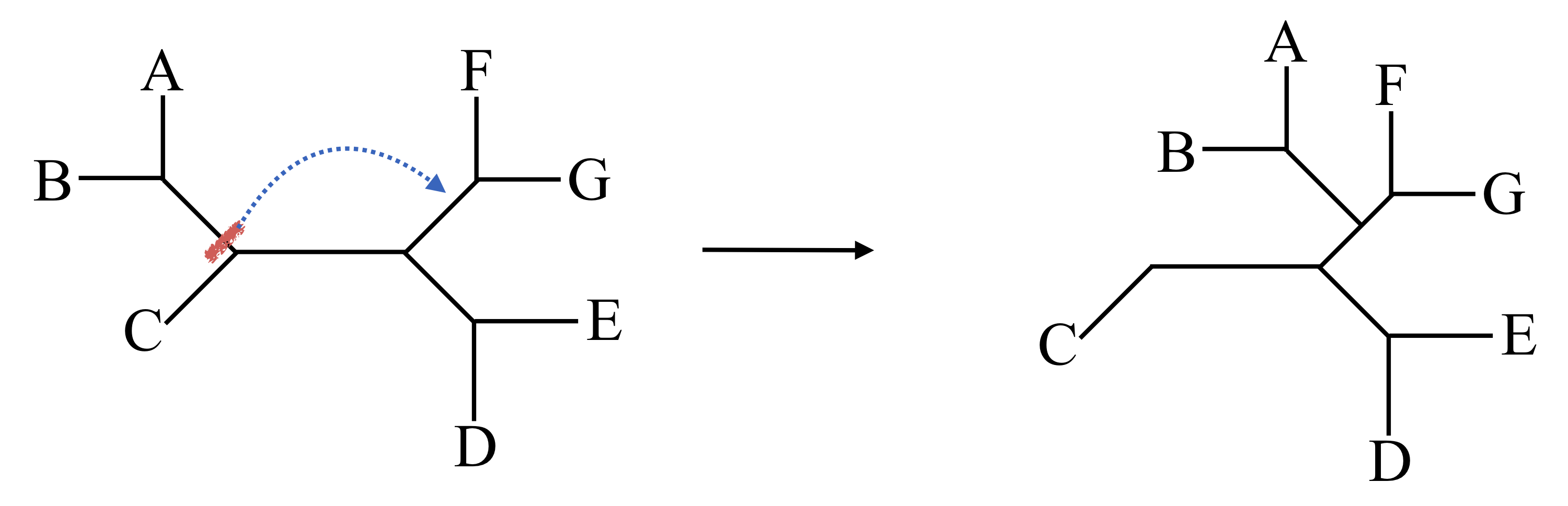
In a SPR move, we lop off any subtree at a node and reattach it somewhere else. Since we have $O(n)$ choices of subtrees to prune off, and $O(n)$ choices of edges to regraft onto, the number of SPR moves is $O(n^2)$ . For large $n$ this means some sort of strategy of which SPR moves to use may be necessary.

SPR example

Distance methods

Many phylogenetic methods have been devised which use a matrix of distances between the taxa to create a tree. These distances are now usually derived somehow from sequence data, for example from the Jukes-Cantor or more sophisticated DNA models considered in Part 1. We will consider two of the simplest methods, UPGMA and Neighbor-Joining.

UPGMA method

The simplest hierarchical clustering/tree-building method using distance data is the UPGMA method, which is almost an acronym for Unweighted Pair Group Method with Arithmetic mean (I am not sure why it isn't the UPGMAM method). At each step in the UPGMA method, the two clusters $C_i$ and $C_j$ with minimum mean distance to each other are joined into a new cluster. The distance from this new cluster, $C_{i,j}$ , to a remaining cluster $C_{k}$ is

$d_{C_{i,j}, C_{k}} = \dfrac{1}{|C_{i,j}| |C_k |} \sum_{a \in C_{i,j}} \sum_{b \in C_k} d(a,b)$

When computing a hierarchical clustering using UPGMA, it is more efficient to compute the distances from a new cluster $C_{i,j}$ (formed from clusters $C_i$ and $C_j$ ) to the remaining clusters using previously computed distances using the formula:

$d_{C_{i,j}, C_{k}} = \frac{|C_i|d_{C_i,C_k} + |C_j|d_{C_j,C_k}}{|C_i| + |C_j|}$

The UPGMA method is simple and fast, but suffers from major problems if the rate of evolution differs along different branches of the tree (see the exercises for a concrete example of this). Therefore the neighbor-joining method, described below, is much more popular as it provides a nice balance between accuracy and speed.

Example of UPGMA

Lets compute the UPGMA clustering for a small distance matrix:

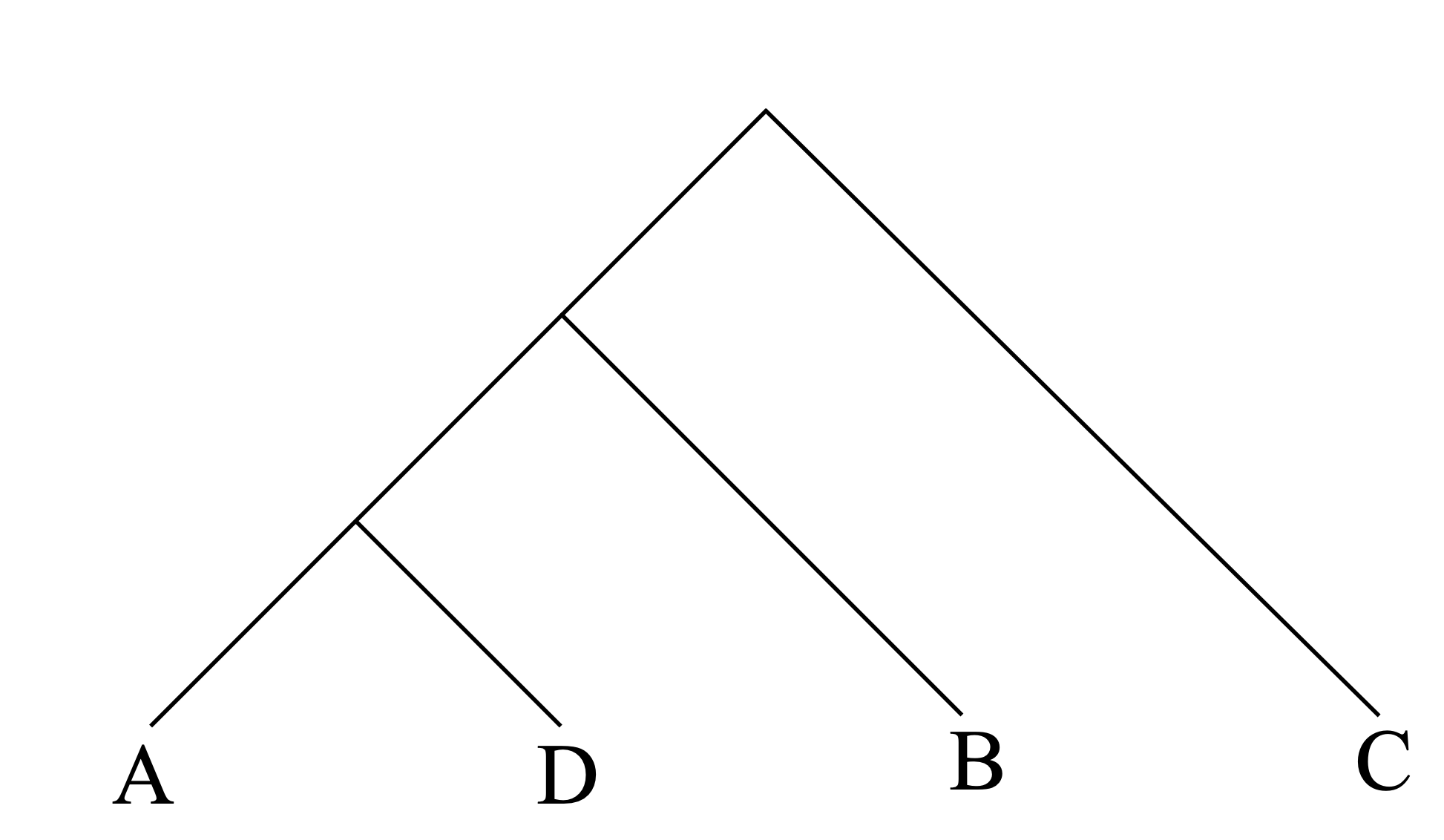
$\left( \begin{array}{ccccc} & A & B & C & D \\ A & 0 & 6 & 8 & 4 \\ B & 6 & 0 & 12 & 8 \\ C & 8 & 12 & 0 & 8 \\ D & 4 & 8 & 8 & 0 \\ \end{array} \right )$

There is a unique minimum, between node $A$ and node $D$ . So we begin by grouping $A$ and $D$ together and then we can compute a new distance matrix

$\left( \begin{array}{cccc} & AD & B & C \\ AD & 0 & 7 & 8 \\ B & 7 & 0 & 12 \\ C & 8 & 12 & 0 \\ \end{array} \right )$

Now the two closest nodes are $(AD)$ and $B$ , so our clustering looks like

Neighbor-joining

The neighbor-joining method was proposed by Saitou and Nei in 1987; it was subsequently analyzed and the implementation improved by several authors, most notably Studier and Keppler in 1988. The survey by Gascuel and Steel in 2006 is an excellent summary if you wish to learn more about the details. It is a somewhat curious algorithm with a relatively complicated history.

The method is iterative; at each stage we join two nodes (taxa or internal tree nodes) into a new node, and compute the distances of the other nodes to the new one. We choose to combine the two nodes $i$ and $j$ which minimize the quantity

$d_{i,j} - r_i - r_j$

where $$r_i = \sum_{k} d_{i,k}/(N-2). $$

The distances to the new node $n$ are given by $$d_{i,n} = d_{i,j}/2 + \frac{1}{N-2}\sum_{k} (d_{ik} - d_{jk})/2= (d_{i,j} + r_i - r_j)/2. $$ $$d_{j,n} = d_{i,j}/2 + \frac{1}{N-2}\sum_{k} (d_{jk} - d_{ik})/2= (d_{i,j} - r_i + r_j)/2. $$ $$d_{n,k} = (d_{i,k} + d_{j,k} - d_{i,j})/2 $$

where $k$ is a node other than $i$ or $j$ .

To illustrate how neighbor-joining is superior to UPGMA we will compute a small example. Suppose we have the set of distances between four entities shown:

$\left( \begin{array}{ccccc} & A & B & C & D \\ A & 0 & 6 & 8 & 4 \\ B & 6 & 0 & 12 & 8 \\ C & 8 & 12 & 0 & 8 \\ D & 4 & 8 & 8 & 0 \\ \end{array} \right )$

First we calculate the $r_i$ :

$r_A = (6 + 8 + 4)/2 = 9$

$r_B = (6 + 12 + 8)/2 = 13$

$r_C = (8 + 12 + 8)/2 = 14$

$r_D = (4 + 8 + 8)/2 = 10$

Now we can calculate the six quantities $d_{i,j} - r_i - r_j$ :

$d(A,B) - r_A - r_B = 6 - 9 -13 = -16$

$d(A,C) - r_A - r_C = 8 - 9 -14 = -15$

$d(A,D) - r_A - r_D = 4 - 9 -10 = -15$

$d(B,C) - r_B - r_C = 12 - 13 -14 = -15$

$d(B,D) - r_B - r_D = 8 - 13 -10 = -15$

$d(C,D) - r_C - r_D = 8 - 14 -10 = -16$

We have tie between the pairs $(A,B)$ and $(C,D)$ . We can arbitrarily choose to join $A$ and $B$ together. Now we can calculate the distance to the $AB$ node to $C$ and $D$ :

$d(AB,C) = (d(A,C) + d(B,C) - d(A,B))/2 = (8 + 12 - 6)/2 = 7$

$d(AB,D) = (d(A,D) + d(B,D) - d(A,B))/2 = (4 + 8 - 6)/2 = 3$

so our updated distance matrix is

$\left( \begin{array}{cccc} & AB & C & D \\ AB & 0 & 7 & 3 \\ C & 7 & 0 & 8 \\ D & 3 & 8 & 0 \\ \end{array} \right )$

Note that if we were using the UPGMA method, nodes $A$ and $D$ would be joined together first, resulting in a different clustering and even in a different unrooted tree topology.

For the final clustering step, $N$ is now $3$ . We recalculate the $r_i$ :

$r_{AB} = 7 + 3 = 10$

$r_C = 7 + 8 = 15$

$r_D = 3 + 8 = 11$

and now

$d(AB,C) - r_{AB} - r_C = 7 - 10 -15 = -18$

$d(AB,D) - r_{AB} - r_D = 3 - 10 -11 = -18$

$d(C,D) - r_C - r_D = 8 - 15 -11 = -18$

This triple tie is not an accident, and reflects the fact that there is only one unrooted tree for three nodes.

The unrooted tree generated by the neighbor-joining algorithm is shown below:

The UPGMA method would have first joined nodes A and D together, which would be incorrect for this tree. Note that the distances along the tree shown are perfectly compatible with the distance matrix.

The neighbor-joining algorithm will perfectly reconstruct a tree if the distance matrix is exactly derived from that tree; it will also reconstruct the correct tree topology for distance data which is only slightly perturbed from a given tree. However, it is not necessarily optimal in general. It is widely used because it often succeeds in practice and it is faster than any of the superior alternatives.

Exercises:

For the distance matrix shown below between the five taxa $A$ , $B$ , $C$ , $D$ , and $E$ , construct unrooted trees using both the UPGMA and neighbor-joining methods. Explain how the two answers differ.

$\left( \begin{array}{cccccc} & A & B & C & D & E \\ A & 0 & 6 & 7 & 10 & 15 \\ B & 6 & 0 & 5 & 8 & 13 \\ C & 7 & 5 & 0 & 7 & 12\\ D & 10 & 8 & 8 & 0 & 7 \\ E & 15 & 13 & 12 & 7 & 0 \end{array} \right )$

Parsimony methods

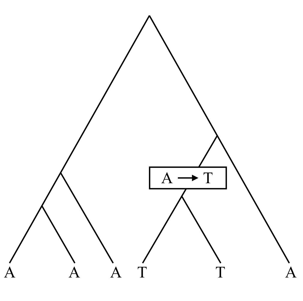
Parsimony methods are based on the principle that the simplest explanation is usually best; in the phylogenetic context this means we are searching for the tree topology which requires the fewest total number of subsitutions in the sites from DNA or protein alignments.

There are several dynamic programming algorithms to compute the parsimony score of a tree. We will examine the Sankoff algorithm for weighted parsimonious trees. In weighted parsimony we can use a cost matrix $c_{ij}$ between states; the simplest cost matrix would be $c_{i,j} = 1$ for $i \neq j$ and $c_{i,i} = 0$ . At tips, costs are infinite or 0. Then compute cost of character $i$ at node $a$ with child nodes $r$ and $l$ as

$S_a(i) = min_j \left (c_{ij} + S_l(j) \right ) + min_k \left (c_{ik} + S_r(k) \right ).$

As an example, consider nucleotide sequence sites, where transitions cost 1 and transversions cost 3. Suppose we have five sites (usually there would be at least thousands of sites for real data):

  1      A   A   G   C   A
  2      A   C   G   C   C
  3      A   C   G   A   A
  4      G   A   C   G   G
  5      A   T   C   G   T

The first column is considered an uninformative site, since every possible 5 taxa bifurcating tree will have a cost of 1 associated with that site. If all of the letters in a column were the same, that would also be an uninformative site.

For the other columns, the goal is to find a single tree that minimizes the total cost (summed over all of the sites). To illustrate the algorithm, lets consider the following tree:

For column 1, the cost is 1, as already mentioned.

For column 2, there are letters A,C,C,A,T in the respective leaf nodes. We start at the lowest nodes (closest to the leaves). At node $A$ , the left branch from node 4 has the letter A, and the right branch has a T. The minimal costs for the letters A,G,C,T at node $A$ are respectively $(3,4,4,3)$ . Similarly, at node $C$ the left and right branches have an A and a C, and the cost of having A,G,C, or T at node C is $(3,4,3,4)$ .

At node $B$ , we use the costs at node $A$ , plus the costs of transitions from those letters, and at the cost of transitioning from the C at node 3. The minimal costs for letters A,G,C, or T at node $B$ are then $(3+3,3+4,0+4,1+3) = (6,7,4,4)$ . Finally (for column 2) the costs of each letter at node $D$ are $(9,11,7,8)$ . The lowest cost is for C, with a cost of $7$ , so column 2 would contribute $7$ to the total cost of the tree.

Now we consider column 3, with letters G,G,G,C, and C. In this case one might guess that the minimal cost will be for letter G at the root node D, but for completeness we list the costs for each letter (in order A,G,C,T) at each node:

Node A: $(6,6,0,2)$

Node B: $(4,3,3,4)$

Node C: $(2,0,6,6)$

Node D: $(5,3,6,7)$

So column 3 has a cost of $3$ .

For column 4, with letters C,C,A,G,G, the costs for letters (A,G,C,T) at each node are:

Node A: $2,0,6,6)$

Node B: $(1,1,6,6)$

Node C: $(6,6,0,2)$

Node D: $(4,4,4,5)$

Node D has a minimal cost of $4$ .

For column 5, with letters A,C,A,G,T, node C has costs $(3,4,3,4)$ (we can reuse the computation from column 2), node A has costs $(4,3,4,3)$ , node B has costs $(4,4,7,6)$ , and node D has costs $(7,8,10,9)$ . So the minimal cost is 7.

Finally, we want to sum all of the costs for each site: the total parsimony cost of this tree for this data is $1 + 7 + 3 + 4 + 7 = 22$ .

The Fitch algorithm provides similar results to the Sankoff algorithm; although superficially different, it is still a dynamic programming algorithm.

Exercises:

First guess a good parsimonious tree for species 1, 2, 3, 4, and 5 from the multiple alignment. Then evaluate the score of this tree using a cost matrix of 3 for a transversion and 1 for a transition (A-to-G or C-to-T) and the Sankoff algorithm. You can save some effort by first grouping sites in to categories, and by calculating the cost of uninformative sites without using the Sankoff algorithm.

Species
```
  1      A   G   C   C
  2      T   C   C   C
  3      A   G   A   C
  4      A   G   T   C
  5      T   C   T   T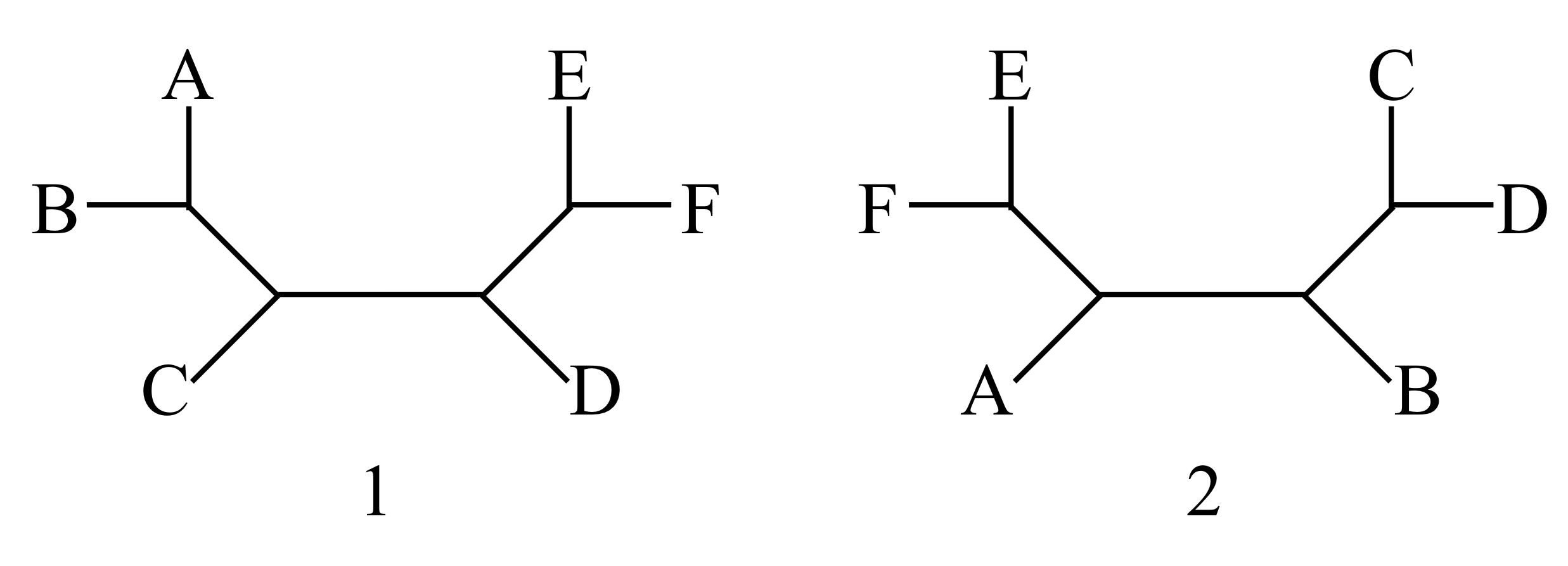
```
What is the minimal number of subtree pruning-and-regrafting (SPR) operations needed to change tree 1 into tree 2? Describe the required operations.
What is the minimal number of nearest-neighbor interchanges (NNIs) needed to change tree 1 into tree 2? Describe one such minimal sequence.
Consider the set of all unrooted trees with five leaves ( $A$ , $B$ , $C$ , $D$ , and $E$ ). Consider two graphs, in both of which each tree is a vertex. In the first graph, connect any two trees which differ by one SPR operation. In the second graph, connect any two trees which differ by one NNI. Describe these graphs as well as you can.

Distance methods

Given a set of taxa, we can compare features ('characters') between every pair of members. In molecular phylogenetics these features will usually consist of DNA or protein sequences. If we can quantify the difference between the features, for example by using a sequence alignment score, then we can obtain a matrix of distances between every pair. The goal of phylogenetic distance methods is to use these distances to reconstruct a tree.

Note that an unrooted tree with $n$ leaves has $2n-3$ edges, so for a given tree topology the problem of determining the edge lengths from the $\displaystyle \frac{n(n-2)}{2}$ distances between pairs is over-determined for $n > 3$ .

Least-squared error methods

A conceptually simple approach is to ask for a tree whose edge lengths are as consistent as possible with the distance data, i.e. a tree which minimizes

$\sum (d_{a,b} - t_{a,b})^2$

where $d_{a,b}$ is the given distance between taxon $a$ and taxon $b$ , and $t_{a,b}$ is the distance within the tree (the sum of the edge lengths connecting $a$ and $b$ ). This criteria tends to over-weight the effects of larger distances, which are typically the least reliable due to alignment artifacts. Therefore Fitch and Margoliash proposed instead minimizing

$\sum \frac{(d_{a,b} - t_{a,b})^2}{d_{a,b}^2} .$

Although not widely used, the Fitch and Margoliash procedure is implemented in the PHYLIP package. The neighbor-joining algorithm, discussed later in this section, is more popular because it gives similar results and is considerably faster. However, for difficult cases with a moderate number of taxa it could be useful to check the results of the Fitch and Margoliash procedure.

In practice one of the most common distance methods used is neighbor joining, described in Chapter 4{reference-type="ref" reference="fast"}. The UPGMA method described in Chapter 4{reference-type="ref" reference="fast"} should not usually be used in phylogenetics because of its tendency to get the wrong tree topology.

Maximum likelihood and Bayesian methods

This lecture provides a good overview of maximum likelihood and Bayesian methods in phylogenetics, and the contrasts between them.

Maximum likelihood

Instead of the somewhat ad hoc approach of parsimony, maximum likelihood methods attempt to find the phylogenetic tree which best matches a probabilistic model for sequence evolution. For DNA, a model such as the HKY + gamma distributed rates could be used.

As with all methods that try to choose the best tree under some criterion, it is computationally expensive to search the tree space exhaustively and for large numbers of taxa it will be impossible. Dynamic programming algorithms for evaluating the likelihood of a model for a given tree exist, although they are somewhat more expensive than the parsimony method.

Bayesian methods

The following example is a good illustration of how Bayesian methods can be superior to maximum likelihood, although it is a little artificial in that we assume we have solid knowledge of the prior, which is usually not the case.

Example. Suppose that there is a disease (such as AIDS or a type of cancer) for which there is a simple test. The test correctly identifies people who have the disease 99% of the time, but also gives a false positive in people who do not have the disease 2% of the time. The disease is fairly rare, however: your doctor says that only about 1 person in 25,000 has it. If you get tested for the disease and the test is positive, what is the chance that you have the disease?

For a positive test result, the maximum likelihood answer is that you probably have the disease. But if we take into account the disease's rarity, we can estimate the chance more accurately. Let $P(P|D) = 0.99$ the probability of testing positive ( $P$ ) while having the disease ( $D$ ), $P(N|D) = 0.01$ the chance of testing negative while having the disease, $P(P|H) = 0.02$ the chance of testing positive while healthy (not having the disease), and $P(N|H) = 0.98$ the chance of testing negative while healthy. We also estimate that $P(H) = \frac{24999}{25000} = 0.99996$ , and $P(D) = 0.00004$ . What we really want to know is $P(D|P)$ , the chance of having the disease if we test positive. By Bayes' rule, this can be computed:

$P(D|P) = \frac{P(P|D)P(D)}{P(P|D)P(D) + P(P|H)P(H)} = \frac{0.99 \times 0.00004}{0.99 \times 0.00004 + 0.02 \times 0.99996 } \approx 0.002$

which implies that we only have a $1$ in $500$ chance of actually having the disease if we test positive (!). This example should be somewhat disturbing.

Phylogenetic invariants

A given tree topology induces certain relations between the probabilities of different patterns character data on the leaves, which can be independent of the branch length. These can be used in principle to distinguish between tree topologies, although so far these methods have had difficulty scaling to large data sets.

We will illustrate the idea with a very simple example, using the Jukes-Cantor model. However it is important to note that the identity we derive holds much more generally. Consider four taxa, $A$ , $B$ , $C$ , and $D$ , and just two of the three possible tree topologies:

For the first tree, $((A,B),(C,D))$ , the Jukes Cantor model gives the following probabilities for differences between taxa; here $P_{AB}$ denotes the probability that taxa $A$ and $B$ differ:

$P_{AC} = \frac{3}{4} - \frac{3}{4} e^{-4\alpha (d_1 + d_3 + d_4)}$

$P_{AD} = \frac{3}{4} - \frac{3}{4} e^{-4\alpha (d_1 + d_3 + d_5)}$

$P_{BC} = \frac{3}{4} - \frac{3}{4} e^{-4\alpha (d_2 + d_3 + d_4)}$

$P_{BD} = \frac{3}{4} - \frac{3}{4} e^{-4\alpha (d_2 + d_3 + d_5)}$

and we see that $(P_{AC} - 3/4)(P_{BD}-3/4) - (P_{BC}-3/4)( P_{AD}-3/4) = 0$ independently of branch lengths.

For the second tree topology,

$P_{AC} = \frac{3}{4} - \frac{3}{4} e^{-4\alpha (d_1 + d_2)}$

$P_{AD} = \frac{3}{4} - \frac{3}{4} e^{-4\alpha (d_1 + d_3 + d_5)}$

$P_{BC} = \frac{3}{4} - \frac{3}{4} e^{-4\alpha (d_2 + d_3 + d_4)}$

$P_{BD} = \frac{3}{4} - \frac{3}{4} e^{-4\alpha (d_4 + d_5)}$

and $(P_{AC} - 3/4)(P_{BD}-3/4) - (P_{BC}-3/4)( P_{AD}-3/4)$ will not be zero for nonzero $d_3$ .

Research into phylogenetic invariants has grown rapidly in recent years.

Population genetics and the coalescent

Previously we considered probabilistic models of DNA subsitutions appropriate to comparisons between species, in which usually enough time has elapsed that it is quite likely that some sites experience multiple substitutions. If we look within a population at the genetic variation between individuals, the situation is quite different. Often it is useful to make the assumption that any difference between sites arises from a single substitution.

The presentation in this chapter is inspired by the book Coalescent Theory, by John Wakeley; it is highly recommended for more depth on this topic.

The times of the branches in a such a genealogical tree (measured from the present), $T_i$ , can be described precisely in the standard coalescent model. This model makes some important assumptions about a population:

The population is constant in size.
The population is panmictic - i.e. well-mixed, without geographic or other barriers.
Substitutions are neutral, having no effect on the fitness of individuals.

While these assumptions do not hold exactly in reality, the basic model can modified appropriately and generally the conclusions we obtain are robust to small deviations from the assumptions. For example we can use a population size that fits the data rather than the actual, experimental population size; this is called the effective population size, often denoted $N_e$ . In human population genetics the effective population size is usually estimated to be about $7,500$ , a million times smaller than the current $7.4 \times 10^9$ . This is the result of population bottlenecks and deviations from the panmictic assumption.

Under these assumptions, in the limit as the number of sites goes to infinity, the standard coalescent model is that the coalescent times $T_i$ are exponentially distributed (see section 16.1.2) with parameter

$\lambda = \left ( \begin{array}{c} i \\ 2 \end{array} \right ):$

$p_{T_i}(t_i) = \left ( \begin{array}{c} i \\ 2 \end{array} \right ) e^{- t_i \left ( \begin{array}{c} i \\ 2 \end{array} \right )}$

with $t_i \ge 0$ and $i \in \{2, \ldots, n \}$ . The expected value and variance are then

$E[T_i] = \dfrac{2}{i(i-1)}$

$V[T_i] = \left ( \dfrac{2}{i(i-1)} \right )^2.$

Note that this means the standard deviation is equal to the expected value, a somewhat counterintuitively large uncertainy.

We can easily compute the expected value and variance of another quantity of interest: the time to the Most Recent Common Ancestor, $T_{MRCA} = \sum_{i=2}^n T_i$ :

$E[T_{MRCA}] = \sum_{i=2}^{n} E[T_i] = \sum_{i=2}^{n} \frac{2}{i(i-1)} = 2 \left (1 - \frac{1}{n} \right ).$

$V[T_{MRCA}] = \sum_{i=2}^{n} V[T_i] = \sum_{i=2}^{n} \left ( \frac{2}{i(i-1)} \right )^2 = 8 \sum_{i=2}^{n} \frac{1}{i^2} - 4 \left ( 1 - \frac{1}{n} \right )^2$

The expected value of the total length of branches ( $T_{total}$ ) in the tree slowly diverges as a function of $n$ :

$E[T_{total}] = \sum_{i=2}^{n} E[i T_i] = \sum_{i=2}^{n} \frac{2}{i-1} \approx \log(n) + \gamma$

where $\gamma$ is the Euler-Mascheroni constant.

Aligned sequences from a population are often studied through some summary statistics, such as:

$S$ , the number of polymorphic sites
$n$ , the number of sequences
$\pi = \frac{2}{n(n+1)} \sum_{i<j} d_{ij}$ , the average number of pairwise differences between sequences, in which $d_{ij}$ is the number of differences between sequence $i$ and sequence $j$ .
$\eta_i$ , the site-frequency spectra. For each $i$ between 1 and $\lfloor n/2 \rfloor$ , $\eta_i$ is the number of sites with $i$ of one letter (base) and $(n-i)$ of another letter.

Here is an example of some human haplotypes; its a subset of the mitochondrial data used in a paper, 'The historical spread of Arabian Pastoralists to the eastern African Sahel evidenced by the lactase persistence -13,915*G allele and mitochondrial DNA' by Priehodova et al. in 2017.

    CAACCAAAC
    CGACCAAAC
    CGGCCAAAC
    CGGCCGAAC
    TAGCCAAAC
    TAGCCGAAC
    TAGCTAAAT
    TAGCTAAGC
    TAGCTAGAT
    TGGCCAAAC
    TGGCTAAAC
    TGGGCAAAC

In this example, $S=9$ , $n=12$ , $\eta_1 = \eta_2 = 3$ , $\eta_3=\eta_5=0$ , $\eta_4=2$ , and $\eta_6 = 1$ .

Tajima's D

Tajima's $D$ -test is a widely used statistical test for the null hypothesis that sites evolve neutrally in a constant-size population. Under the null hypothesis, the expected value of the two quantities $\pi$ and $S/a_1$ should be equal, where $$a_1 = \sum_{i=1}^{n-1} \frac{1}{i}. $$

If the null hypothesis were true, we would expect that the coefficient of variation of $d = \pi - S/a_1$ would be small, usually between $0$ and $1$ . Tajima's $D$ -test studies a signed version of the coefficient of variation, denoted $D$ :

$D = \frac{d}{Var(d)} = \frac{\pi - \frac{S}{a_1}}{e_1S + e_2S(S-1)}$

where $\displaystyle a_2 = \sum_{i=1}^{n-1} \frac{1}{i^2}$ and

$e_1 = \frac{c_1}{a_1} \ \ \ \ e_2 = \frac{c_2}{a_1^2 + a_2}$

in which

$c_1 = b_1 - \frac{1}{a_1} \ \ \ \ c_2 = b_2 - \frac{n+2}{a_1 n} + \frac{a_2}{a_1^2}$

which in turn need

$b_1 = \frac{n+1}{2(n-1)} \ \ \ \ b_2 = \frac{2(n^2 + n +3)}{9n(n-1)}.$

If $D$ is not between $-2$ and $2$ , it constitutes strong evidence that the null hypothesis is false.