Interpolation

The interpolation problem is: given a set of pairs of values $(x_i, y_i)$ for $i \in (0,N+1)$ , find a function $p(x)$ within a particular class (usually polynomials) such that $p(x_i) = y_i$ .

In this section we will only consider polynomial interpolation, but other sorts of functions can be very useful as well, such as rational or trigonometric functions. For polynomial interpolation we will choose the lowest-degree polynomial that interpolates the points. For $N+1$ points, as long the x-values are distinct the interpolating polynomial will be degree $N$ .

Direct solving with Vandermonde matrices

The simplest approach to interpolation is to write the interpolating polynomial as

$p(x) = a_0 + a_1 x + a_2 x^2 + \ldots + a_{N} x^{N}$

and set up a linear system for the unknown coefficients $a_i$ :

$\left(\begin{array}{cccc} 1 & x_0 & x_0^2 & \ldots & x_{0}^{N} \\ 1 & x_1 & x_1^2 & \ldots & x_{1}^{N} \\ \vdots & \vdots & \vdots & \vdots & \vdots \\ 1 & x_N & x_N^2 & \ldots & x_{N}^{N} \end{array} \right ) \left(\begin{array}{c} a_0 \\ a_1 \\ \vdots \\ a_N \end{array} \right ) = \left(\begin{array}{c} y_0 \\ y_1 \\ \vdots \\ y_N \end{array} \right )$

The coefficient matrix is called a Vandermonde matrix, named after Alexandre-Theophile Vandermonde, an 18th-century mathematician and violinist.

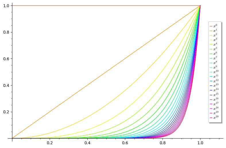
As the number of interpolation points increases, the Vandermonde matrix becomes ill-conditioned, and solving for the coefficients becomes difficult to do accurately. This is a reflection of the fact that we are using powers of $x$ as our basis; these powers get less and less independent in some sense as $n$ gets larger. Consider the figure below, of the first 21 powers of $x$ , and notice how they become almost indistinguishable on the interval $[0,1]$ .

Example: Lets consider a degree $N$ interpolating polynomial at the points $x_i = -1 + 2i/N$ for $i \in \{0,1,\ldots,N\}$ . The condition number of the Vandermonde matrix $V$ is about 40,000 for N=10, but quickly increases to $7.73 \cdot 10^{16}$ for $N=35$ . This large condition number means that in directly solving the linear system we are apt to lose many digits of precision (possibly all of them for a 64-bit float).

Lagrange interpolation.

This method of interpolation uses a polynomial basis adapted to the choice of interpolation points:

$\displaystyle p(x) = \sum y_i \frac{\prod_{j\neq i} (x - x_j)}{\prod_{j\neq i} (x_i-x_j)} = \sum y_i l_i(x)$

The basis polynomials $l_i(x)$ have the convenient properties that $l_i(x_i) = 1$ , and $l_i(x_j) = 0$ if $i \neq j$ . They are often referred to as Lagrange polynomials, or the Lagrange basis, but this is a bit of a misnomer as they were described earlier by Waring in 1779, and by Euler in 1783, before Lagrange's 1795 publication using them.

There some more efficient ways to write these polynomials. For a given set of interpolation points $x_i$ , let $\phi = \prod_i (x-x_i)$ , and then

$l_i = \frac{\phi(x)}{(x-x_i)\phi'(x_i)}$

which is a useful form for using complex analysis to study interpolation polynomials. We can evaluate the interpolation polynomial more efficiently if we precompute some of the quantities in it. In particular, if we let

$\lambda_i = \frac{1}{\phi'(x_i)} = \frac{1}{\prod_{j\neq i} (x_i-x_j)}$

then we can write

$p(x) = \phi(x) \sum_i \frac{y_i \lambda_i}{x - x_i}$

This is already pretty efficient but we can do even better by using the fact that

$\sum_i l_i(x) = 1$

which means that we can write

$l_i(x) = \left ( \frac{\lambda_i}{x - x_i} \right ) / \left ( \sum_j \frac{\lambda_j}{x - x_j} \right )$

and this common denominator in the formula for $p(x)$ gives us:

$p(x) = \left ( \sum_i \frac{y_i \lambda_i}{x - x_i} \right ) / \left ( \sum_i \frac{\lambda_i}{x - x_i} \right )$

which is called the barycentric form of Lagrange interpolation.

Below is an interactive example of Lagrange interpolation for 4 movable points. The polynomial $p(x)$ is in black, and the four basis polynomials $l_1(x), l_2(x), l_3(x), l_4(x)$ are in red, blue, purple and green.

Lagrange Interpolation Example

Use the Lagrange basis to find the interpolating polynomial for the points $(0,0)$ , $(1,1)$ , $(2,-1)$ , and $(3,3)$ .

If we use the original form (the barycentric form is not really necessary for this small example), we have the four Lagrange polynomials

$l_0 = \frac{(x-1)(x-2)(x-3)}{(0-1)(0-2)(0-3)} = 1 - 11 x/6 + x^2 - x^3/6$

$l_1 = \frac{(x-0)(x-2)(x-3)}{(1-0)(1-2)(1-3)} = 3 x - 5 x^2/2 + x^3/2$

$l_2 = \frac{(x-0)(x-1)(x-3)}{(2-0)(2-1)(2-3)} = -3 x/2 + 2 x^2 - x^3/2$

$l_3 = \frac{(x-0)(x-1)(x-2)}{(3-0)(3-1)(3-2)} = x/3 - x^2/2 + x^3/6$

and the interpolating polynomial is

$p(x) = (0) l_0 + (1) l_1 + (-1) l_2 + 3 l_3 = 11 x/2 - 6 x^2 + 3 x^3/2$

Newton's Divided Differences Interpolation

We now turn to a different technique of constructing interpolants, which is often called "Newton's divided differences", but Isaac Newton was not the first to invent these. The true inventor appears to be Thomas Harriot, who among many other accomplishments introduced divided differences in a work on algebra in the early 1600s. (Harriot has also been credited as the first observer of sunspots, introducing the potato to Ireland, discovering the law of refraction ("Snell's Law"), and performing precise observations of Halley's Comet that later lead to an accurate orbit determination by Bessel.) Harriot's interest in triangular calculations is also related to the Bezier curves we will examine later.

A divided difference depends on a function $f$ and a set of $n+1$ points $x_0, \ldots, x_n$ , and is denoted as $f[x_0,x_1,\ldots,x_n]$ . They are defined recursively as follows:

$f[x_0] = f(x_0)$

$f[x_0,x_1] := \frac{f[x_1] - f[x_0]}{x_1 - x_0}$

$f[x_0,x_1,\ldots,x_n] := \frac{f[x_1,x_2,\ldots,x_n] - f[x_0,x_1,\ldots,x_{n-1}]}{x_n - x_0}$

These quantities are the coefficients of the interpolating polynomial in the Newton basis $1, (x-x_0), (x-x_0)(x-x_1), \ldots$ , so

$p(x) = f[x_0] + f[x_0,x_1] (x-x_0) + f[x_0,x_1,x_2] (x-x_0)(x-x_1) + \\ \ldots + f[x_0,x_1,\ldots,x_N] (x-x_0)(x-x_1)\ldots (x-x_N)$

interpolates the points $(x_0, f(x_0))$ , $(x_1, f(x_1))$ , $\ldots$ , $(x_N, f(x_N))$ .

The primary advantage of the divided differences method of interpolation is that a new interpolation point can be added with only $O(N)$ extra computation. The divided differences are also important in their own right since they are approximations to derivatives of $f$ , and are useful in interpolation error estimates (next section).

Divided differences have some interesting properties:

They are totally symmetric in their arguments, i.e. if $\sigma$ is a permutation of $\{0,1,\ldots,N \}$ , then $f[x_0,x_1,\ldots,x_N] = f[x_{\sigma(0)}, x_{\sigma(1)}, \ldots, x_{\sigma(N)}]$ . This can be proved by an inductive argument.
Divided differences of products of functions follow a Leibniz rule:

$(f g)[x_0,x_1,\ldots,x_N] = \sum_{r=0}^{N} f[x_0,x_1,\ldots,x_r] g[x_r,x_1,\ldots,x_N]$

Divided differences satisfy a generalization of the mean-value theorem: for some $z$ contained in the smallest interval containing all of the $x_i$ ,

$f[x_0,x_1,\ldots,x_{N}] = \frac{f^{(N)}(z)}{N!}$

This will be proved below as part of an interpolation error estimate theorem.

For a given set of points $x_0,x_1,\ldots,x_N$ , we can associate to any function $f$ a matrix $T_f$ :

$T_f = \left ( \begin{array}{ccccc} f[x_0] & f[x_0, x_1] & f[x_0, x_1, x_2] & \ldots & f[x_0, \ldots, x_N] \\ 0 & f[x_1] & f[x_1, x_2] & \ldots & f[x_1, \ldots, x_N] \\ \vdots & \vdots & \ddots & \vdots & \vdots \\ 0 & \ldots & 0 & f[x_{N-1}] & f[x_{N-1}, x_N] \\ 0 & 0 & 0 & \ldots & f[x_N] \end{array} \right )$

and these matrices form a commutative ring, with $T_{f g} = T_f T_g$ . This means they are simultaneously diagonalizable. The common diagonalizing matrix of eigenvectors is

$S = \left ( \begin{array}{cccccc} 1 & \frac{1}{(x_1-x_0)} & \frac{1}{(x_2-x_0)\cdot(x_2-x_1)} & \frac{1}{(x_3-x_0)\cdot(x_3-x_1)\cdot(x_3-x_2)} & \ldots & \frac{1}{\prod_{j=0}^{N-1} (x_N - x_j)} \\ 0 & 1 & \frac{1}{(x_2-x_1)} & \frac{1}{(x_3-x_1)\cdot(x_3-x_2)} & \ldots & \frac{1}{\prod_{j=1}^{N-1} (x_N - x_j)} \\ 0 & 0 & 1 & \frac{1}{(x_3-x_2)} & \ldots & \frac{1}{\prod_{j=2}^{N-1} (x_N - x_j)} \\ \vdots & \vdots & \vdots & \ddots & \ddots & \vdots\\ 0 & 0 & 0 & \ldots & 1 & \frac{1}{(x_N-x_{N-1})} \\ 0 & 0 & 0 & \ldots & 0 & 1 \end{array} \right )$

The expanded form: if we write a divided difference with the $y_i$ as separate coefficients, we obtain the "expanded form", which makes some of their symmetry properties much more obvious:

$f[x_0, x_1, \ldots, x_n] = \sum_{i=0}^n \frac{y_i}{(x_i - x_0)\ldots(x_i - x_n)}$

where the products in the denominator do not include the terms which would be zero (i.e. $(x_i - x_i)$ ).

Error estimates and bounds

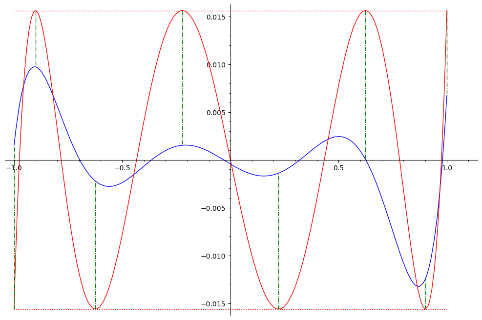
The mathematician and physicist Carl Runge found a surprisingly extreme example of the failure of polynomial interpolants to approximate the function

$f(x) = \frac{1}{1 + 25 x^2}$

when using a uniform subdivision of the interval $(-1,1)$ . The coefficient 25 in the function is not essential; any similar function causes similar problems. In the figure below, a series of interpolating polynomials on increasingly fine uniform grids is shown. As the number of interpolation points is increased, the deviation of the interpolating polynomial from $f(x)$ increases dramatically near the endpoints.

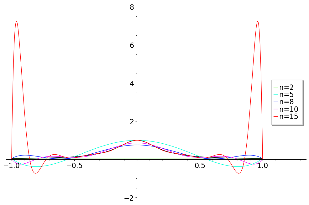
Runge example — Runge's example of convergence failure.

This example inspired Runge and others to carefully examine the interpolation error.

The main theorem in this regard is:

If $p(x)$ interpolates $f(x)$ at the $N+1$ points $x_0, \ldots, x_{N}$ and $f(x)$ has $N+1$ bounded derivatives on the interval $[a,b]$ containing the $x_i$ , then for each $x$ in $[a,b]$ there is a point $z \in [a,b]$ such that

$f(x) - p(x) = \frac{f^{(N+1)}(z)}{(N+1)!} \prod_{i=0}^{N} (x - x_i)$

The proof of this result also gives us a generalization of the mean value theorem for divided differences:

Proof of the interpolation error formula

Let $P(x)$ be the interpolating polynomial for a $\mathcal{C}^{N+1}$ function $f(x)$ at the points $x_0 < x_1 \ldots < x_{N-1} < x_{N}$ . At a point $x_{N+1}$ , the error $P(x_{N+1}) - f(x_{N+1})$ can be found by considering the the polynomial $Q(x)$ that interpolates $f$ at $x_0, x_1, \ldots, x_{N+1}$ . Using the Newton basis, we have

$P(x_{N+1}) - f(x_{N+1}) = f[x_0,x_1,\ldots,x_{N+1}] (x_{N+1}-x_0) (x_{N+1}-x_1) \ldots (x_{N+1}-x_{N})$

Now if we consider the function

$R(x) = P(x) - f(x) - f[x_0,x_1,\ldots,x_{N+1}] (x-x_0) (x-x_1) \ldots (x-x_{N})$

we know it has $N+2$ zeros at $x_0, x_1, \ldots, x_{N+1}$ . By Rolle's theorem, this means that $R'(x)$ has $N+1$ zeros between the zeros of $R(x)$ . Similarly $R''(x)$ has $N$ zeros in between those zeros of $R'(x)$ , and we can continue in this way until we arrive at the fact that $R^{(N+1)}(x)$ has a zero at $z$ which is somewhere between the largest and smallest of the $x_i$ . Since $P(x)$ is only a degree $N$ polynomial, its $N+1$ th derivative is zero, and

$R^{(N+1)}(z) = f^{(N+1)}(z) - (N+1)! f[x_0,x_1,\ldots,x_{N+1}] = 0$

$f[x_0,x_1,\ldots,x_{N+1}] = \frac{f^{(N+1)}(z)}{(N+1)!}$

The error bound suggests a general strategy for minimizing the error, which leads us to Chebyshev points and polynomials.

Chebyshev points and polynomials

Chebyshev polynomials arise in a number of mathematical contexts but for our purposes they can be viewed as a way to elegantly minimize the part of the interpolation error that comes from the grid points, i.e. as a way to minimize $|\phi_N(x)|$ on the interval $[-1,1]$ where

$\phi_N(x) = (x-x_0)(x-x_1)\ldots (x - x_N)$

If we wish to interpolate a function $f$ on a different interval $[a,b]$ , we can construct an interpolant $p(x)$ for $g(x) = f((x(b-a) + a+b)/2)$ on $[-1,1]$ , and then rescale it to $q(x) = p((2x-a-b)/(b-a))$ .

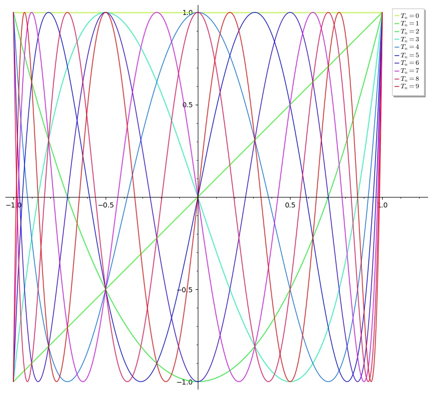
The Chebyshev polynomials are defined as $T_{n} = \cos(n \arccos(x))$ . (The use of the letter T here comes from the French transliteration of Chebyshev's name as Tchebycheff.) The first few are easy to compute directly from this definition:

$T_0(x) = 1$

$T_1(x) = x$

$T_2(x) = 2 x^2 - 1$

$T_3(x) = 4 x^3 - 3 x$

$T_4(x) = 8 x^4 - 8 x^2 + 1$

Using the angle-addition trigonometric identities it is straightforward to find the recurrence relation:

$T_{n+1}(x) = 2xT_n(x) - T_{n-1}(x)$

which shows that the $T_n$ are indeed polynomials. They have many known properties.

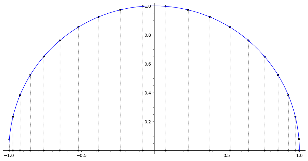
Chebyshev functions — The first 10 Chebyshev polynomials.

The Chebyshev points (for a given $n$ ) are defined as the zeros of $T_n(x)$ . Since $\cos(\theta)$ is zero at any odd multiple of $\pi/2$ , the Chebyshev points for each $n$ are $x_i = cos(\frac{k \pi}{2 n})$ where $k \in \{1,3,\ldots,2n - 1 \}$ . These are the vertical projections of uniformly spaced points on the unit circle.

Chebyshev points as projections — Chebyshev points for n=20.

In proving the optimality of the Chebyshev points, it is convenient to use a monic version of $T_n(x)$ which is $M_n(x) = 2^{-n+1}T_n$ . The fact that the leading coefficient of $T_n$ is $2^{n-1}$ (for $n>0$ ) can be proved from the recurrence relation $T_{n+1}(x) = 2xT_n(x) - T_{n-1}(x)$ .

We need a few more facts about the $T_n$ for the optimality proof. From the recurrence relation $T_{n+1}(x) = 2xT_n(x) - T_{n-1}(x)$ and the base cases $T_0 = 1$ and $T_1 = x$ we can prove by induction that $T_n(1) = 1$ and $T_n(-1) = (-1)^{n}$ . More generally, at $x = cos(\frac{k \pi}{2 n})$ for even integers $k$ , $T_n(x)$ will alternate between $1$ and $-1$ . The monic version $M_n$ will alternate between $2^{-n+1}$ and $-2^{-n+1}$ at those same $n+1$ points.

Optimality proof for Chebyshev points

The optimality proof is by contradiction: suppose there is a monic polynomial $q(x)$ of degree $n$ which is always smaller than $2^{-n+1}$ in absolute value on the interval $[-1,1]$ . Consider the difference between $q$ and $M_n$ : $r(x) = M_n(x) - q(x)$ . At the $n+1$ alternating extreme values of $M_n$ , $r(x)$ must have the same sign as $M_n(x)$ , so $r(x)$ changes sign at least $n$ times on the interval $[-1,1]$ . But since both $q$ and $M_n$ are monic, their $n$ th-degree terms cancel out, so $r(x)$ is at most a $(n-1)$ th degree polynomial. By the fundamental theorem of algebra, $r(x)$ can have at most $n-1$ distinct roots unless it is the zero polynomial. To satisfy our assumptions, $r(x)$ is not zero but it has $n$ distinct roots in $[-1,1]$ , which is a contradiction.

Chebyshev optimality proof example — Example components of the optimality proof for n=7, with the monic Chebyshev polynomial in red.

Barycentric form of interpolant with Chebyshev points

The good convergence properties of Chebyshev points mostly arise from the way their spacing decreases near the interval endpoints; if we use the projection of any near-uniformly spaces points on the circle we will get similar convergence properties.

A particular useful case is to use the extreme locations of the Chebyshev polynomials as interpolation points instead of their zeros, i.e. $x_k = \cos((k \pi)/(2n))$ where $k$ is even ( $k=2j$ ) and in $[0,2n]$ . These are sometimes called Chebyshev points of the second kind, or extreme Chebyshev points. With this choice the interpolation weights simplify to $(-1)^j 2^{n-1}/n$ except at the endpoints, where they are half of that. The common factors of $2^{n-1}/n$ cancel out of the interpolation formula, leading to the beautifully simple and efficent formula

$p(x) = \left ( \sum_i' \frac{y_i (-1)^i}{x - x_i} \right ) / \left ( \sum_i' \frac{(-1)^i}{x - x_i} \right )$

where the primed sums indicate that the first and last terms of the sum must be multiplied by 1/2. In Sage this could be implemented by something such as:

def chebint(f,a,b,n):
    '''
    Chebyshev barycentric interpolation
    f = function (of x) to be interpolated
    a,b = interval of interpolation
    n = number of interpolation points
    '''
    npi = float(pi)
    cpts = [(cos(k*npi/(2*n-2))+1)*(b-a)/2 + a for k in range(0,2*n,2)]
    trms = [(-1)^j/(x-cpts[j]) for j in range(0,n)]
    trms[0] = trms[0]/2
    trms[-1] = trms[-1]/2
    top = sum([f(x=cpts[j])*trms[j] for j in range(n)])
    bot = sum(trms)
    return top/bot

Theorems of Faber and Krylov

Chebyshev points are of immense practical utility, as they provide a relatively simple scheme for choosing the interpolating points that have a lot of nice properties. But there are some fiendish functions for which interpolation on Chebyshev points will not converge. Faber's Theorem says that it is impossible to find a fixed scheme for which the interpolant will always converge, if we allow any continuous functions as the class of functions we wish to interpolate.

More happily, a theorem of Nikolay Krylov guarantees the convergence of any absolutely continuous function on a bounded interval if the Chebyshev points are used. So the vast majority of functions which arise in applications will not have convergence problems.

Hermite, Fejer

When interpolating a differentiable function, it is sometimes desirable to match the derivatives of $f$ as well as its values at the interpolation points. In Hermite interpolation the interpolating polynomial matches the value and the first $m$ derivatives of the given $f$ (often the term Hermite interpolation is only used for $m=1$ ). The divided differences method can be reused here, with repeating values of the $x_i$ interpolation points. A repeated $x_i$ gives an undefined divided difference, but the limit as interpolation points coalesce is well-defined as a derivative of $f$ as long as $f$ is smooth enough at that point.

Natural cubic splines

When designing curved shapes for projects such as ship hulls, drafters and builders of the past used thin flexible rods often pinned or anchored in place by weights. Using low degree (usually cubic) piecewise polynomial curves gives a very similar mathematical set of tools called splines. We will start with one of the more useful types of splines, the `natural' cubic splines.

$s_i(x) = y_i + b_i (x - x_i) + c_i (x - x_i)^2 + d_i (x - x_i)^3$

for which we require that the $s_i, s_i', s_i''$ match with $s_{i+1}, s_{i+1}', s_{i+1}''$ respectively at each interior point, and $s''(x_1)=s''(x_n) = 0$ . It is the latter endpoint conditions that distinguish natural splines.

A major advantage of splines is that unlike in global interpolation there is no problem in using uniformly spaced interpolation points. For evenly spaced $x_i$ , let $\Delta_i = y_{i+1} - y_i$ , $h = x_{i+1} - x_i$ . Then using the smoothness and interpolation conditions we can write the $b_i$ and $d_i$ in terms of the $d_i$ :

$b_i = \Delta_i/h - \frac{h}{3}(2 c_i + c_{i+1})$

$d_i = \frac{c_{i+1} - c_i}{3 h}$

The natural spline conditions mean that we can set $c_0 = c_n = 0$ (we don't actually find a polynomial $s_n(x)$ , but its convenient in writing the formulas to have a $c_n$ ), and then solve for the interior $c_i$ by solving the linear system

$\left ( \begin{array}{ccccc} 4 & 1 & 0 & \ldots & 0 \\ 1 & 4 & 1 & \ldots & 0 \\ 0 & 1 & 4 & \ldots & 0 \\ \vdots & \vdots & \ddots & \ddots & \vdots \\ 0 & \ldots & 0 & 1 & 4 \end{array} \right ) \left ( \begin{array}{c} c_1 \\ c_2 \\ \vdots \\ \vdots \\ c_{n-1} \end{array} \right ) = \left ( \begin{array}{c} 3 y[x_0, x_1, x_2] \\ 3 y[x_1, x_2, x_3] \\ \vdots \\ \vdots \\ 3 y[x_{n-2}, x_{n-1}, x_n] \end{array} \right )$

where

$y[x_i, x_{i+1}, x_{i+2}] = \frac{y_{i+2} - 2 y_{i+1} + y_i}{h^2}$

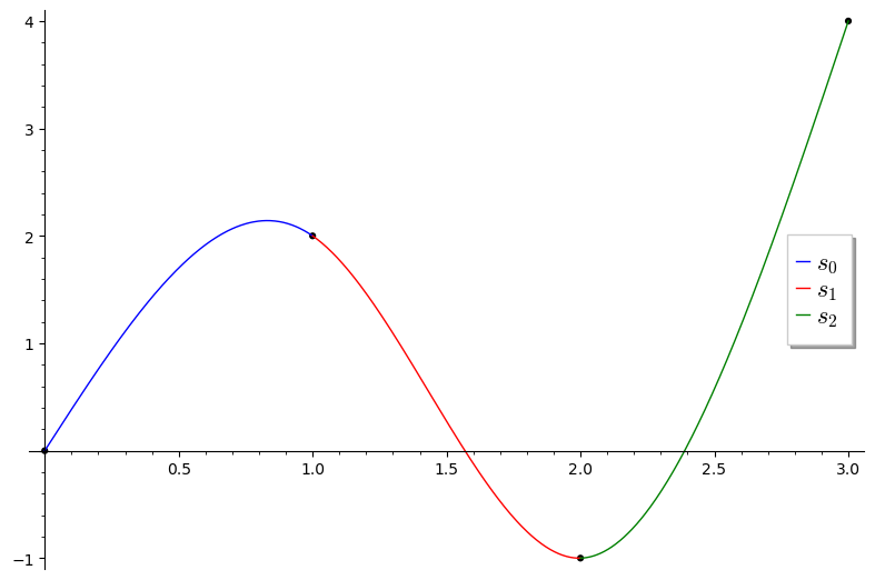
Example natural spline

Lets compute the natural spline through the points $(0,0)$ , $(1,2)$ , $(2,-1)$ , and $(3,4)$ . These are uniformly spaced with $x_{i+1} - x_i = h = 1$ . To find $c_1$ and $c_2$ we need to solve the system

$\left ( \begin{array}{cc} 4 & 1 \\ 1 & 4 \end{array} \right ) \left ( \begin{array}{c} c_1 \\ c_2 \end{array} \right ) = \left ( \begin{array}{c} 3 \frac{y_{2} - 2 y_{1} + y_0}{h^2} \\ 3 \frac{y_3 - 2 y_2 + y_1}{h^2} \end{array} \right ) = \left ( \begin{array}{r} -15 \\ 24 \end{array} \right )$

The solution to this is $c_1 = -\frac{28}{5}$ , $c_2 = \frac{37}{5}$ . We can now solve for the $d_i$ and $b_i$ :

$d_0 = \frac{c_{1} - c_0}{3 h} = -\frac{28}{15}$

$d_1 = \frac{c_{2} - c_1}{3 h} = \frac{13}{3}$

$d_2 = \frac{c_{3} - c_2}{3 h} = -\frac{37}{15}$

$b_0 = (y_1 - y_0)/h - \frac{h}{3}(2 c_0 + c_1) = (2-0)/1 - \frac{1}{3}(0 -\frac{28}{5}) = \frac{58}{15}$

$b_1 = (y_2 - y_1)/h - \frac{h}{3}(2 c_1 + c_2) = -3 - \frac{1}{3}(2 \frac{-28}{5} + \frac{37}{5}) = -\frac{26}{15}$

$b_2 = (y_3 - y_2)/h - \frac{h}{3}(2 c_2 + c_3) = 5 - \frac{1}{3}(2 \frac{37}{5} + 0) = \frac{1}{15}$

and our three polynomials are

$s_0(x) = \frac{58}{15} x - \frac{28}{15} x^3$

$s_1(x) = 2 - \frac{26}{15}(x-1) - \frac{28}{5}(x-1)^2 \frac{13}{3}(x-1)^3$

$s_2(x) = -1 + \frac{1}{15}(x-2) + \frac{37}{5}(x-2)^2 - \frac{37}{15}(x-2)^3$

which are shown below in blue, red, and green respectively.

Bezier curves

In many design settings we actually desire corners and sharp transitions, at least as an option. For this more varied design goal it is common to use parameterized splines called Bezier curves. These were developed in the 1950s in industrial settings (the automobile companies Renault and Citroen) independently by engineers Pierre Bezier and Paul de Casteljau.

A key difference between Bezier curves and the natural cubic splines considered earlier is that there is no required matching of derivatives between different segments, allowing sharp corners. This is often desirable in design applications (such as creating fonts).

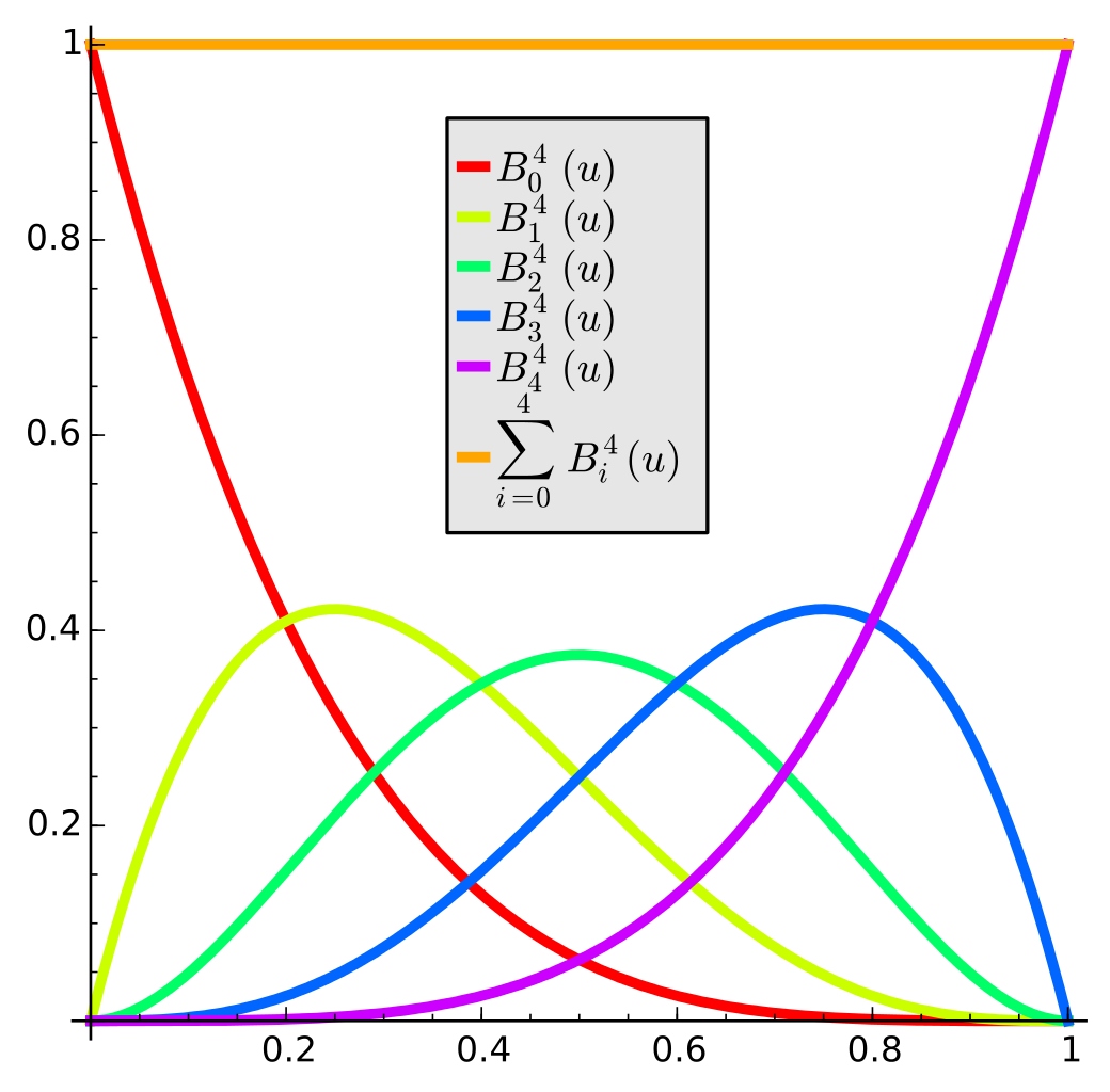
There are several different ways to define and compute Bezier curves. We will define them as a kind of weighted average of $N+1$ vector points $P_0$ , $P_1$ , $\ldots$ , $P_N$ . The weights will come from a binomial partition of unity:

$1 = 1^N = ((1 - t) + t)^N = (1-t)^N + {N \choose 1} t (1-t)^{N-1} + \ldots$

$+ {N \choose i} (1-t)^{N-i} t^i + \ldots + {N \choose N-1} t^{N-1} (1-t) + t^N$

Recall that the binomial coefficients are defined as

${N \choose i} = \frac{N!}{i!(N-i)!}$

The polynomial terms in the sum are often called Bernstein polynomials:

$B_i^N(t) = {N \choose i} (1-t)^{N-i} t^i$

These polynomials are useful for many other things in polynomial analysis; for example they are used in a proof (by the eponymous Bernstein) of the Weierstrass approximation theorem:

For any function $f$ that is a continuous on an interval $[a,b]$ , and any $\epsilon > 0$ , there exists a polynomial $P$ such that

$max_{x \in [a,b]} |P(x) - f(x)| < \epsilon$

We use each Bernstein polynomial in the sum to weight the points, so the Bezier curve is

$P(t) = (1-t)^N P_0 + {N \choose 1} t (1-t)^{N-1} P_1 + \ldots + {N \choose N-1} t^{N-1} (1-t) P_{N-1} + t^N P_N$

This works for points $P_i$ in any dimension, but they are most commonly used in the plane. In fact, the text you are reading right now is drawn with letters that are defined by Bezier curves.

The famous binomial identity from Pascal's triangle:

${N \choose i} = {(N-1) \choose i} + {(N-1) \choose (i-1)}$

gives rise to a corresponding identity of Bernstein polynomials:

$B_i^N(t) = (1-t) B_i^{N-1}(t) + t B_{i-1}^{N-1}(t)$

This identity in turn enables a recursive construction of Bezier polynomials, the de Casteljau algorithm.

The introduction of these curves in industrial design was simultaneously pioneered by Pierre Bezier at the car company Renault, and Paul de Casteljau at Citroën, in the late 1950s and early 1960s. They are now used ubiquitously in design and other applications, including type fonts, animation, robotic motion planning, and sound design.

Exercises

Use the Lagrange form to find the interpolating polynomial of the points $(-1,-2)$ , $(1,1)$ , and $(2,3)$ .
Find the interpolating quadratic for $\sin(x)$ at $x = 0$ , $x=\frac{\pi}{6}$ , and $x=\frac{\pi}{2}$ .
What is the relative error of the interpolating quadratic at $x=\frac{\pi}{3}$ ?
Use the divided differences method to calculate the interpolating polynomial $p_h(x)$ that passes through $y = \cos(x)$ at $x = 0$ , $x=h$ , and $x=2h$ .
Compute $\lim_{h \rightarrow 0} p_h(x)$ .
If $P(x)$ is a polynomial of degree 3, and $Q(x)$ is a polynomial of degree 4, is it possible for $P(x)$ and $Q(x)$ to intersect in exactly 5 points? If so, give an example; if not, explain why not.
For the interpolation points $x_1 = -a$ , $x_2 = a$ , with $a \in [0,1]$ , find the value of $a$ which minimizes the maximum of the absolute value of $\phi(x) = (x - x_1)(x - x_2)$ on the interval $[-1,1]$ .
Compute the 'natural' (zero second derivatives at the endpoints) cubic spline that interpolates the points $(0,-8)$ , $(1,1)$ , and $(2,4)$ . It may be easiest to use the polynomial basis $\{ 1$ , $(x-1)$ , $(x-1)^2$ , $(x-1)^3 \}$ for this particular problem.