
Nonlinear Systems
Nonlinear systems and linearizations at equilibria
First the bad news: the vast majority of nonlinear systems of differential equations do not have explicit solutions (in terms of elementary functions such as trigonometric functions, polynomials, and exponentials), and in general are very difficult to analyze. However there are a wide variety of methods to at least partially analyze the solutions. This chapter will focus on one of the most important techniques which leverages what we have already learned about linear systems: linearizing near an equilibrium.
For a system of ODEs:
where x and F(x) are n-dimensional vectors, the equilibria are the values of x for which F(x) = 0. These will be constant solutions. Near these equilibria the slope function F will be small and not too different from its linear approximation, as long as F is 'nice' (e.g. continuously differentiable). The main idea is to replace F with its linearization, giving us a linear system that will reflect the nonlinear solution near that equilibrium.
We will only consider systems in 2 or 3 dimensions, but the idea extends to any number of dimensions. Let's start with the 2-D case.
In 2-D we can rewrite the general nonlinear system more explicitly in terms of its components:
The equilibria are the points (x_1,x_2) where both f_1(x_1, x_2) = 0 and f_2(x_1, x_2) = 0. Such a nonlinear algebraic system may already be difficult (or even impossible) to solve explicitly; we will only consider problems where it is possible to find the equilibria. Let's call one such equilibrium point p = (p_1, p_2).
We want to linearize the slope function F(x), which means linearizing the components f_1(x_1,x_2) and f_2(x_1,x_2). The graph of each of these functions is surface in 3D; the linearization at p is the tangent plane of that surface at p. For each f_i we can calculate the tangent plane by combining the tangent lines in the x_1 and x_2 directions:
The tangent plane to f_i at p is the graph of L_i. In vector-matrix form, we can combine these two linearizations:

This looks just like a 1-D tangent line, but DF_p is a matrix of derivatives instead of just a scalar slope. The matrix DF_p is called the Jacobian of F at p, named after the famous 19th century mathematican Carl Jacobi.
If we shift our coordinates to be centered at p with u = x - p, then the linearized system is
and we can analyze this using our linear methods (the eigenvalue/eigenvector method or the Laplace transform).
As usual, this should be clearer if we look at a particular example.
Example
We will find the equilibria and their linearizations for the system:
The equilibria will the solutions to x_1 + x_2 = 0 and 1 - x_1^2 = 0. In general we usually want to eliminate variables until we have an equation in just one variable; here we already have such a single-variable equation: 1 - x_1^2 = 0. It has two solutions, x_1 = \pm 1. If we substitute those values of x_1 into the first equation we find that x_2 = - \pm x_1, where the plus and minus is the same as for x_1 - i.e. the variables x_1 and x_2 need to have opposite signs to solve the equilibrium equations. So we have two equilibria, (1,-1) and (-1,1).
The Jacobian of our system is
For the first equilibrium point (1,-1) our linearized system is
where u_1 = x_1 - 1 and u_2 = x_2 + 1. We can determine the behavior of the linearized system by finding the eigenvalues and eigenvectors of the coefficient matrix. The eigenvalues are roots of
The quadratic formula gives us the complex roots \lambda = \frac{1}{2} \pm i \sqrt{\frac{7}{2}}. Complex roots with a positive real part such as these mean that the linearized system will expand in a swirling motion, so the equilibrium is unstable. The fact that the first column of the coefficient matrix is (1,-2)^T means that if we are slightly to the right of the equilibrium we will be moving down and to the right, so the solution is spiralling outwards in a clockwise direction. This gives us a good qualitative description of the linearization without needing to compute the explicit solution.
The other equilibrium (-1,1) is superficially similar but the sign change in its Jacobian has important effects. For it, u_1 = x_1 + 1 and u_2 = x_2 - 1, and the linearization is
The characteristic polynomial is
with roots
These real roots mean that there is one eigenline (the span of an eigenvector) along which the linearized solution expands exponentially (e^{2t}), and another eigenline on which it contracts exponentially (e^{-t}). So this equilibrium is also unstable, with most nearby solutions having some exponential expansion.
Some trajectories of the full nonlinear system are shown below.

And here is an animated version:
Exercises:
-
Find the equilibria of the system x' = x y /2 - 4, y' = x - 2y.
-
Find the eigenvalues of the linearized system at each equilibria. Determine whether each equilbrium is stable or unstable.
The trace-determinant plane
- The eigenvalues of a two by two matrix A depend on all of its four entries. Let's examine exactly how this dependence works by computing the characteristic equation for a general A:
From this we see that the eigenvalues only depend on the trace of A (the sum of its diagonal elements) and the determinant of A:
The eigenvalues are have a nonzero imaginary part if and only if the discriminant \text{tr}(A)^2 - 4 \det(A) is negative - a parabola in the trace-determinant plane for two by two matrices. Below is an interactive animation of the flow of solutions to a system x' = Ax, where you can control the trace and determinant of A with the sidebar's circle.
Exercises:
-
Construct a two by two matrix A with zero trace and positive determinant (try to make it as simple as possible).
-
What are its eigenvalues and eigenvectors?
-
Sketch the solutions to the system x' = Ax for your matrix (where x = \left ( \begin{array}{c} x_1 \\ x_2 \end{array} \right )).
-
For the family of initial values problems x_1(0) = 0, x_2(0) = 1, and x' = Ax where
A = \left ( \begin{array}{cc} 1 & 1 \\ 0 & a \end{array} \right )find the solution x(t) assuming that a>0, and then compute \lim_{a \rightarrow 1} x.
Population dynamics: Lotka-Volterra equations
In the 1920s, the Italian mathematician Vito Volterra was told by his son-in-law of some curious changes in the fish population of the Adriatic Sea; during World War I it was much less safe to fish the Adriatic, which resulted in a shift of species and sizes of fish caught after the war. Volterra came up with a simple system of ODEs which could at least partly explain the fishermen's observations. Volterra's equations are essentially identical to other equations that were developed around the same time by the American mathematician Alfred Lotka. This famous system is usually referred to as the Lotka-Volterra equations in their honor.
The system models two species, one of which preys on the other. We will denote the prey species population by x, and the predator population by y. The model assumes that the predators catch the prey at a rate proportional to x y, which is the same assumption as in the law of mass action used in modeling the rate of chemical reactions (which Lotka also modeled). There are parameters b (birth rate of prey), p, q, and d (death rate of predators), all of which are positive. The system is:
To analyze the system we begin by finding the equilibria (critical points) by setting these rates of change to 0:
From the first equation we can see that either x=0 or y=b/p.
If x=0, then the second equation requires that either y=0 or x = d/q. But since we assumed x=0, we have only the equilibrium (0,0).
If y=b/p, then in the second equation y cannot be 0, and x=d/q. So we have a second equilibrium at (d/q, b/p).
The Jacobian matrix of derivatives of the slope field is
At the first equilibrium (0,0) the Jacobian simplifies to
Since this is diagonal we can immediate see that (1,0) and (0,1) are eigenvectors with eigenvalues b and -d. This equilibrium is unstable because of the positive eigenvalue b.
At the second equilibrium (d/q, b/p) the Jacobian becomes
The characteristic equation for this matrix is
so the eigenvalues are \pm i \sqrt{bd}. When we have purely imaginary eigenvalues such as this, the linearized equations are stable (barely!) with elliptic solutions around the equilibrium, but it is unclear if the nonlinear system is stable or not. In this particular system it turns out that the equilibrium is surrounded by periodic orbits and it is stable.
Some of the periodic orbits for parameters b=d=q=p=1 are shown below.

Exercise

We will consider a model of the populations of moose (m) and wolves (w) on Isle Royale. In the absence of wolves, assume the moose population will follow the logistic equation (m' = km(P-m)) with some carrying capacity P. The wolves will deplete the moose population at a rate proportional to their product (amw for some a > 0). The wolf population will die off at a rate -dw for some d>0 in the absence of moose, and increase at a rate bmw for some b>0. So the model is
If t is in years, then k is approximately \frac{1}{5000}.
-
Find the equilibria of the system in terms of k,P,a,b, and d.
-
Estimate reasonable values of P,a,b, and d based on the data shown above.
-
For your choices of parameters, is the equilibrium with positive m and w stable or unstable?
The Lorenz equations
In the early 1960s, Edward Lorenz developed a model for atmospheric convection which in its simplest form can be written as:
This is now referred to as the Lorenz system of ODEs. This system possesses many interesting properties, including the existence of a "strange attractor" and chaotic dynamics for some values of the parameters. The computer modeling necessary to really see its complicated behavior was first done by Ellen Fetter working with Lorenz.
One viewpoint on the system with \beta=8/3, \rho=28, and \sigma=10 is shown below. There was
Exercise
-
Find the eigenvalues of the Lorenz system linearized at the origin (x,y,z) = (0,0,0). For what values of \sigma>0, \rho>0, and \beta>0 is the origin unstable? The Lorenz system is:
x' = \sigma (y - x)y' = x(\rho - z) - yz' = x y - \beta z
Hopf Bifurcations
In two dimensions there is an important common type of bifurcation of equilibria known as the Hopf bifurcation. In this type of bifurcation, as a parameter is varied an equilibrium changes its stability type and a periodic solution is created around it.
As an example of a Hopf bifurcation, consider the following system in variables x and y, with parameter b:
which is a particular (simplified) case of the 1968 Selkov model for glycolysis; the variables x and y are related to the concentrations of the chemicals ADP and ATP in a cell. For each b there is a unique equilibrium at x = b, y = \frac{10 b}{(10 b^2 + 1)}. The Jacobian of the system is
which at the equilibrium becomes
The eigenvalues are the somewhat intimidating functions of b:
In the Selkov model, b is a positive parameter. Between b \approx 0.016 and b \approx 2.38, the discriminant is negative, and there are complex eigenvalues. When b < \sqrt{\frac{4 - \sqrt{5}}{10}} \approx 0.42, or b > \sqrt{\frac{4 + \sqrt{5}}{10}} \approx 0.79, the real part of the eigenvalues is negative and the equilibrium is stable. When b is in the interior of the interval (0.42, 0.79), the equilibrium is unstable but there is stable periodic orbit around it.
An animation from Wikipedia of these bifurcations is shown below.

Exercise:
-
Convert the system
\frac{dx}{dt} = ax + y - x(x^2 + y^2)\frac{dy}{dt} = -x + ay - y (x^2 + y^2)to system for r' and \theta ' in polar coordinates r, \theta. For r = \sqrt{x^2 + y^2} it is easiest to use the squared relation r^2 = x^2 + y^2 and differentiate with respect to t; for \theta we can compute the derivative through the implicit relation \tan(\theta) = \frac{y}{x} or the explicit \theta = \arctan{(y/x)}.
-
Solve the polar differential equations and sketch the solutions for a = -1 and a = 1.
Limit Cycles: The Van der Pol Oscillator
The Van der Pol oscillator is a nonlinear ODE featured in a famous paper by Mary Cartwright and John Littlewood in 1945. It is also related to models of oscillation in musical reed instruments such as clarinets introduced by Lord Rayleigh. One form of this ODE is:
This is a homogeneous linear ODE; it is also commonly studied with periodic forcing.
We can get a sense of the behavior of the solutions with some numeric approximations. From the (1 - x^2) term it seems there is an important natural scale to the ODE, so lets use initial conditions with (x(0,x'(0)) = (1/2,0), (1,0), (2,0), and (4,0). We will use the second-order improved Euler method as an example, and use the parameter value \mu = 1.
First we convert the 2nd-order ODE to a system of first-order equations:
We can package this into a vector system
with
and
Now at each step we can update an approximation X_i to
where h is the stepsize. For the picture below we used 1000 steps, from t=0 to t=20.

The only equilibrium of the Van der Pol system is at (0,0). The Jacobian there is
which has the characteristic equation \lambda^2 - \lambda + 1 with eigenvalues
Since the real parts of the eigenvalues are positive, the origin is an unstable spiral. However we can see that these outwardly spiralling solutions converge on a periodic solution. This system has a limit cycle, a periodic solution that is approached by other solutions. In fact for the Van der Pol system it is possible to prove that every solution other than the constant (0,0) solution approaches this limit cycle.
Additional and review exercises
-
Solve the initial value problem x'' + 2x' + 5x = t, x(0) = 0, x'(0) = 0, and find the exact value of x(2).
-
Rewrite the ODE as a first order system.
-
Approximate the solution x(2) using two steps of the Euler method. Compare this with an approximation using one step of the Improved Euler Method, and to the exact value.
The Improved Euler method is: k_1 = f(t_n,\vec{x}_n)
k_2 = f(t_n + h, \vec{x}_n + h k_1)\vec{x}_{n+1} = \vec{x}_n + h (k_1 + k_2)/2t_{n+1} = t_{n} + hFor this problem, \vec{x} = (x, v) where v = x'. Each slope k_i is also a two-component vector, and the function f is vector-valued (i.e. it outputs a two-component vector).
-
Consider an long cascade of tanks, each containing 1 liter of water. Each tank drains into the next at a rate of 1 liter per hour. Initially the first tank contains 1 gram of salt dissolved into it, but it is being refilled with pure water at a rate of 1 liter per hour. The other tanks in the cascade are initially filled with pure water. Compute how much salt is in the nth tank at time t.
-
Compute the inverse of
A = \left[ \begin{array}{rrr} \cos(\theta) & -\sin(\theta) & 0 \\ \sin(\theta) & \cos(\theta) & 0 \\ 0 & 0 & -1 \\ \end{array}\right] -
Are the vectors v_1 = \left ( \begin{array}{r} 1 \\ -1 \\ 0 \\ 0 \end{array} \right ), v_2 = \left ( \begin{array}{r} 0 \\ 1 \\ -1 \\ 0 \end{array} \right ), v_3 = \left ( \begin{array}{r} 0 \\ 0 \\ 1 \\ -1 \end{array} \right ), v_4 = \left ( \begin{array}{r} -1 \\ 0 \\ 0 \\ 1 \end{array} \right ) linearly independent? If not, write one of them as a linear combination of the others.
-
Solve the initial value problem
x' = \left [ \begin{array}{rr} 2 & -5 \\ 1 & -2 \end{array}\right ]x, \ \ \ x(0) = \left [ \begin{array}{r} 2 \\ 1 \end{array}\right ]. -
Sketch the solution.
-
What is the eccentricity of the ellipse?
Additional Exercises
-
Compute the equilibria of the following nonlinear differential equations, and use that information to match each equation with a trajectory plot from the following page. It may be helpful to compute the eigenvalues at the equilibria.
-
x' = x - y, y' = x + 3y - 4.
-
x' = 2x - y, y' = x - 3y.
-
x' = 2 \sin(x) + \sin(y), y' = \sin(x) + 2\sin(y).
-
x' = x - 2y, y' = -x^3 + 4x.
-
x' = 1-y^2, y' = x+2y.
-
x' = x - 2y + 3, y' = x -y +2.
-
-
Find the unique equilibrium of the system x' = x - y, y' = 5x - 3y -2. Compute the eigenvalues of its linearization to determine the stability of the equilibrium (see Theorem 2 in section 9.2).
-
Find the equilibria and the eigenvalues of their linearizations for the system x' = 2x - y - x^2, y' = x - 2y + y^2.
-
In 1958, Tsuneji Rikitake formulated a simple model of the Earth's magnetic core to explain the oscillations in the polarity of the magnetic field. The equations for his model are:
x' = -\mu x + y zy' = -\mu y + (z-a)xz' = 1 - xywhere a and \mu are positive constants. Find the equilibria for this system for a=\mu=1, and determine the stability of the linearized system at those equilibria. It is acceptable to use a computer algebra system such as Sage to compute the eigenvalues of the linearized systems; it may also be helpful to express the equilibria and the Jacobian matrix in terms of the golden ratio, \displaystyle g = \frac{\sqrt{5} + 1}{2} (note that 1/g = g-1).
A 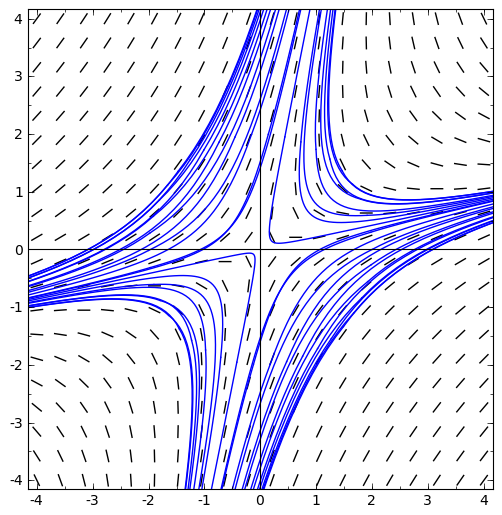
B 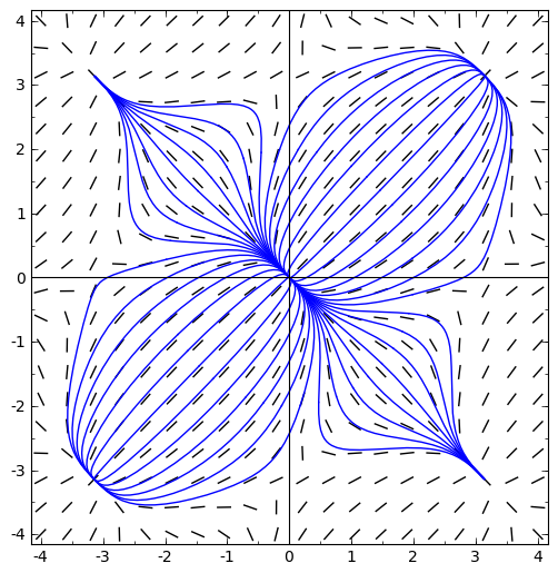
C 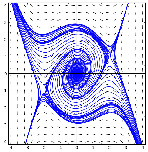
D 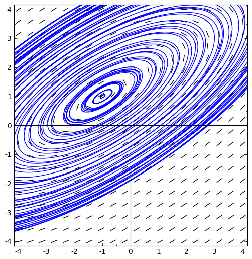
E 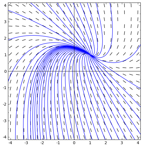
F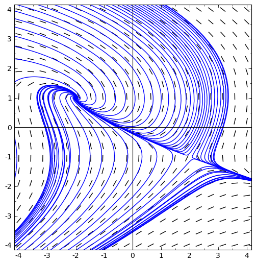
Notes
Notes: (Local storage in a cookie)
License

This work (text, mathematical images, and javascript applets) is licensed under a Creative Commons Attribution-NonCommercial-ShareAlike 4.0 International License. Biographical images are from Wikipedia and have their own (similar) licenses.