EE 2212

Fall 2014

11 September 2014

Experiment 1: RC Circuits-Frequency and Time Domain Response Measurements

Note: Experiment 1 Scheduled For Thursday, 11 September. Report Due Thursday, 18 September, In Lab

LABORATORY NOTEBOOKS AND INFORMATION

Ø Review the Laboratory Information document on the EE 2212 WEB site including the grading rubric.

Ø I want to emphasize that your report is to be no more than three additional pages besides the cover page. This will require that you look at your results with an “engineering eye” to distill and summarize your results.

Ø Every student will keep a patent-style laboratory notebook. Patent-style refers to a numbered page bound notebook. Loose leaf binders are not allowed and would not be legally accepted in a patent filing. Everything you do in lab and related to the lab which includes lab preparation, in-lab discussion, prelabs, data, comments during the lab, etc. are to be included in the notebook.

Ø The notebook is a stand-alone document from which a colleague with similar background and experience would be able to understand and reproduce your results. This means key diagrams, connection diagrams, design equations, etc.

Ø If there are errors or problems encountered in the laboratory, these are also to be included in your notebook so that a colleague could study the approach you took to move to a better approach.

Ø No loose sheets of paper are to be used for data collection.

Ø Date your entries in your notebook. This is a standard practice for IP (Intellectual Property) in a patent style notebook.

Ø You can tape or staple in graphs, screen dumps, SPICE plots, etc and/or alternatively, reference locations where data files, resides should anyone request to see it. (i.e. flash drives, computer files, etc.)

Ø Your notebook is your key working document from which you will use generate high-quality reports. I encourage you to annotate your results with key statements, comments, and conclusions as you proceed though the experiments.

Ø I will review your notebooks periodically through the semester.

Ø If any equipment is not working or if there are no components in the bins, do not keep it a secret. Please let me know so that I can address the problem.

Ø Do not put defective components back in the bins and do not put defective leads and cables back on the cable rack. Give the defective leads to me and I will bring them to the shop for repairs.

NOW TO THE EXPERIMENT

OBJECTIVES

This laboratory is designed to be a review of some key EE 2006 concepts and a review of the lab equipment operation..

Ø Review the operation of the Tektronix TDS 3012B Two-Channel Color Digital Oscilloscope, Tektronix AFG 3021C Function Generator, Fluke 8808A DMM, and Impedance Bridge for measuring capacitor values, and the LAN connected to the oscilloscope, computer, and printer.

Ø There are a number of soft-key nested menus for you to explore on both the oscilloscope and function generator.

Ø Be able to print Tektronix TDS 3012B screens to the networked printer on each bench.

Ø Be able to store Tektronix TDS 3012B screens to your flash drive on the networked computer.

Ø Be able to insert images from SPICE and Tektronix TDS 3012B screens into document files.

Ø Measure and plot the time and frequency domain responses of single section RC circuits.

Ø Apply the RC response to illustrate the concept of a passive element integrator and differentiator in the time domain.

Ø Use SPICE for AC and TRAN simulations to compare with your analysis and measurements.

PRELAB

Ø You must have a patent-style laboratory notebook with you. That is a bound notebook (not looseleaf) with numbered pages.

Ø Review the appropriate EE 2006 material related to first-order time domain system responses and frequency domain impedance concepts. This will be reviewed in lab.

Ø Review SPICE material from EE 2006 so that you will be able to write and run SPICE programs for each of the circuits for this lab. SPICE is also available on the computers in the laboratory and those of you with wireless laptops can also access the network from MWAH 391. Print the waveforms of the inputs and outputs on the same set of axes. You will need to read the entire experiment to be able to understand what is expected and where you will need the SPICE graphs. SPICE will be demonstrated in lab. You will need the following information from your SPICE simulation in order to complete this lab:

· 3 dB BW (bandwidth), t_r (rise time)_,t (time constant), key amplitudes and times

· AC analysis of frequency and phase for the frequency domain

· TRAN analysis for the time domain

PROCEDURE

1. Time Domain First Order System Analysis

Construct the following two circuits on your prototype board. Observe that the circuits are duals of each other.

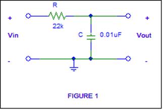
TIME DOMAIN RESPONSE Of Figure 1

Ø Drive Circuit 1 with a 2 volt peak-to-peak square wave and observe the output. You will need to adjust the frequency of the square wave such that key attributes of the waveform are shown for a first-order response. The 2-volt level is not critical. The first order response equation is given by:

where the time constant τ = RC. A is the amplitude of v_in(t).

Ø To measure the time constant t, determine t_63% which is the time required for the output to reach 63% of its final value during a half-cycle of the input. Does it equal the actual value of the RC product for your measured values of the resistors and capacitors you are using? Why or why not? You may need to change the horizontal time scale and vertical gain of the oscilloscope (and the amplitude of the input, if needed) to attain this measurement. Save key waveforms on flash drive. Measure and record the time constant t.

Ø Also, measure the rise time t_rand record. ( t_r= t_90% - t_10%= 2.2t). Finally, compare the theoretical, experimental, and SPICE values of time constant and rise time. Many of these measurements can be done by using settings within the oscilloscope “MEASURE” menu. Fill in the following table. This is a good table to include in your lab report.

Parameter	Calculated	SPICE	Measured	Comments
Rise Time, t_r
Time Constant, τ

Ø Now change the frequency of the input square wave from approximately 1 kHz to 30 kHz and adjust your amplitude appropriately to observe key waveform attributes so that you can observe that this circuit behaves as an analog passive integrator. That is over a limited range,

Ø Now apply a triangular wave to the input of the circuit. Note input and output waveforms, amplitudes and times. Do these measurements agree with the values and expected circuit time response you found using SPICE?

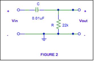
TIME DOMAIN RESPONSE Of Figure 2

Ø Drive Circuit 2 with a 2 volt peak-to-peak square wave (amplitude is not critical) and observe the output. You will need to adjust the frequency of the square wave such that key attributes of the waveform are shown for a first-order response. The first order response equation is given by:

where the time constant τ = RC. A is the amplitude of v_in(t).

Ø To measure the time constant t, determine t_37% which is the time required for the output to reach 37% of A during a half cycle of the input. Does τ = RC for your measured values of the resistor and capacitor you are using? Why or why not? You may need to change the horizontal time scale and vertical gain of the oscilloscope (and the amplitude of the input, if needed) to attain this measurement. Save key waveforms on flash drive. Measure and record the time constant τ.

Ø Also, measure the fall time t_fand record. ( t_f= t_90% - t_10%= 2.2t). Finally, compare the theoretical, experimental, and SPICE values of time constant and rise time. Many of these measurements can be done by using settings within the oscilloscope “MEASURE” menu. Fill in the following table. This is also a good table to include in your lab report.

Parameter	Calculated	SPICE	Measured	Comments
Fall Time, t_f
Time Constant, τ

Frequency Domain Response Of Figure 1 (Low-Pass Filter)

The circuit in Figure 1 is also a basic single-pole analog passive low-pass filter (LPF). This LPF function can be observed by applying a constant-amplitude (i.e. 2 volt peak-to-peak amplitude input sinusoid and varying the frequency from 50 Hz to > 10 kHz.

Ø Measure and record the "low-frequency" (f = 50 Hz) gain and phase shift. Use the magnitude of this gain to measure accurately the – 3 dB corner frequency of the filter, and the phase shift. (Note that –3 dB corresponds to 70.7% of the low-frequency gain). Again, you can obtain phase directly from the “MEASURE” menu and visually verify by looking at the waveforms. Compare these measurements with theoretical and PSPICE values. Many of these measurements can be done by using settings within the oscilloscope “MEASURE” menu. Measure and plot the gain and phase shift at several frequencies out to >10 kHz. Is the high-frequency gain roll-off about –6dB/octave (-20dB/decade) as the frequency is increased? Plot the data as you change the frequency to ascertain the detail you need.

Ø Finally, using SPICE, show a db plot of 20 log |A(jf)| and a phase plot of q (jf) (voltage gain and phase as a function of frequency) of the circuit of Figure 1 Vary the frequency from 50 Hz to >10 kHz. Select data points that show the key features of the curves. This is a good table to include in your lab report.

Parameter	Calculated	SPICE	Measured	Comments
Low Frequency Gain
Low Frequency Phase
3 dB Frequency
Gain at 3 dB Frequency
Phase at 3 dB Frequency

FREQUENCY DOMAIN RESPONSE Of Figure 2 (High Pass Filter)

The circuit in Figure 2 is also a basic single-pole passive high-pass filter. To see this, observe the amplitude of the output as the frequency is varied from >10 kHz down to 50 Hz. You will need to use a 2 volt peak-to-peak constant-amplitude input sinusoid.

Ø Measure the high-frequency (f >10 kHz) gain and phase shift. Use the magnitude of this gain to measure f_c and the phase shift there. Compare these measurements with your PSPICE values.

Ø Measure the gain and the phase shift of the filter at low frequencies. Is the low-frequency gain roll-off about -6dB/octave as the frequency is decreased? Again, Many of these measurements can be done by using settings within the oscilloscope “MEASURE” menu.

Ø Finally, using SPICE, show a plot of 20 log |A(jf)| and q(jf) of the circuit of Figure 2. Vary the frequency from 50 Hz to 10 kHz. Select data points that show the key features of the curves. Again, plot the data as you proceed and change the frequency. This is a good table to include in your lab report.

Parameter	Calculated	SPICE	Measured	Comments
High Frequency Gain
High Frequency Phase
3 dB Frequency
Gain at 3 dB Frequency
Phase at 3 dB Frequency

Now for a little technically appropriate humor.