EE 2212

EXPERIMENT 3

21 February 2013

Diode I-V Measurements and Half Wave and Full Wave Bridge Rectifiers

PURPOSE

Ø Use laboratory measurements to extract key diode model parameters including I_S ,n (also called h or N in SPICE) from the I-V measurements of the 1N4001.

Ø Modify the default (Dbreak) SPICE diode model to reflect your measurements and compare and also compare with the 1N4002 model in SPICE. All specifications except the PRV (PIV) should be similar between the 1N4001 (PRV=50 volts) and 1N4002 (PRV=100 volts).

Ø Implement designs of the half wave rectifier and full wave bridge rectifier circuits and measure time domain characteristics and the transfer characteristics of each.

Ø Measure and compute ripple voltage as a percentage and as an rms value. You can use both the soft-keys on the oscilloscope or the multimeter

Ø Compare individual diode results and circuit results using SPICE simulations.

COMPONENTS

Ø 1N4001 Diodes (Use 1N4002 diode model in SPICE as well as the generic “Dbreak” model)

Ø 1 kW resistors

Ø 0.1 mF, 1mF, and 10mF capacitors Actual values not critical

PROCEDURE

I-V Characteristics and Diode Model Parameter Extraction

Ø Using SPICE, simulate the circuit shown in Figure 1. Obtain the I-V characteristic curve for both the 1N4002 and default Dbreak model in SPICE over a range at least of -0.1 to 0.8 volts and find the diode current value for each diode when v_D = 0.7 volts. For this, it might be useful to use a DC voltage sweep in conjunction with a VDC source. In addition, you will need to change the x-axis

value to be the voltage across the diode (v+) – (v-) under Plot_Axis Settings…_Axis Variable…-

Ø Examine the model characteristics for each the 1N4002 and the Dbreak in PSPICE, which can be

found by selecting the device and then Edit_Model…_Edit Instance Model (Text)…

Ø Construct the circuit. Use two digital multimeters (one to measure I_D and another to measure V_D). You could also use the voltmeter on the power supply and a meter at the cathode and subtract to get the diode voltage. Note the I_D can also be measured by measuring the voltage across the resistor and dividing by R. Pay attention to the diode orientation. The banded side is the cathode end. Change the supply voltage V_DC to adjust I_D to the desired current setting, then measure V_D. Take enough readings to accurately define the diode characteristic. You should measure out to I_D values of a few mA. Record your results in a data table in both your laboratory notebook and in your laboratory report. Consider the equation which approximates to when the diode is forward biased. To facilitate graphing over a number of orders of magnitude we obtain,

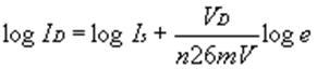Note that log(_{base 10)} e = 0.434

Ø From this equation, determine and fit a straight line (linear regression) to your plotted I-V semi-log graph. Your equation will be in the form y = mx + b

Use these data to modify the default diode (D) model in your SPICE program. Virtually all calculators have the linear regression (least squares linear fit) built-in. Be sure you use this modified default Dbreak model for simulating the laboratory results as well as the 1N4002 model. This is what you essentially did in Text Problem 3.21.

Half-Wave Rectifier

Ø Refer to Figure 2. Change the from VDC to V_Sine as a 10 volt peak-to-peak 100 Hz sinusoid. Perform a SPICE transient analysis simulation and observe the the half-wave rectification. Also note the offset voltage when you compare the input and output waveforms. Observe and plot Vout(t) and the transfer characteristic, Vo vs V_Sine.

Ø Experimentally observe the operation on the oscilloscope in both the time domain and as a transfer function.

Ø Now we want to “smooth out” the pulsating DC by using capacitors.

Ø Place a C across the 1 kΩ resistor. Now use all three values of C to illustrate the change in the ripple voltage by measuring Vout(t). Use the ”Measure” menu on the oscilloscope to measure the rms voltage of the output using dc and ac coupling. Explain the differences in these measurements and explain what these measurements are illustrating. Use your diode model and check your lab measurements using SPICE. Observe that ripple voltage is defined as either the (DV/Vpeak) x 100% or as(Vrms or as Vrms of the output voltage/Vpeak )x 100%. Watch your polarity on the electrolytic capacitors you may use. Also, since electrolytic capacitors have a broad tolerance, their values must be checked on the capacitance meter to obtain accurate results. I will demonstrate the operation of the capacitance meter.

Diode-Bridge Full-Wave Rectifier

Ø Construct the circuit shown in Figure 3. Note that to provide a floating input from the signal generator which has one side grounded , we will use a transformer to provide isolation. Do not monitor the input of the bridge with the oscilloscope because you will automatically ground (that is short circuit) one side of the circuit. Monitor the input on the signal generator side of the circuit. (Brown and blue transformer primary winding). Also observe how this floating input is modeled in SPICE.

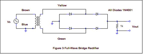
Ø Input Vs as a 10 volt peak-to-peak 100 Hz sinusoid. Observe and plot Vo(t) and the transfer characteristic, Vo vs Vs. Compare your results with what would be expected for an ideal diode bridge. Explain why this circuit would function as an “absolute value” function system.

Ø Now use the three values of C to illustrate and measure the change in ripple voltages by measuring Vo(t). Use the ”Measure” menu on the oscilloscope to measure the rms voltage of the output using dc and ac coupling. Explain the differences in these measurements and explain what these measurements are illustrating. Use your diode model and check your lab measurements using SPICE.

Ø Compare your full-wave rectifier results with the half-wave rectifier circuits.

(An added historical note: The background screen is a photo of a “cat whisker” diode used as an AM radio detector in the 1905-1920 era of early radio before the widespread use of vacuum tubes. A sharp springy wire (cat whisker) formed a pressure junction with a galena crystal. Galena is PbS (lead sulfide) and has a bandgap of about 0.4 eV. Of course, the underlying physics was unknown at the time. Primitive, but it did work-sort of. A reincarnation of this was used by soldiers in World War II in what is called a “foxhole radio”. The junction for detection of strong AM radio signals was a sharp wire contacting a “blue edge razor blade to form a crude junction. The “bluing process on the single edge razor blade of the time creates a difference in the work functions between the wire and the metal razor which results in a rectifying junction.

A Classic