EE 2212

Spring 2017

19 January 2017

Experiment 1: RC Circuits-Frequency and Time Domain Response Measurements

Report Due: Thursday, 26 January in Lab

LABORATORY NOTEBOOKS AND INFORMATION

Ø Review the Laboratory Information document on the EE 2212 WEB site including the grading rubric.

Ø I want to emphasize that your report is to be no more than three additional pages besides the cover page. This will require that you look at your results with what I call an “engineering eye” to distill and summarize your results.

Ø Every student will keep a patent-style laboratory notebook. Patent-style refers to a numbered page bound notebook and the associated electronic files. Loose leaf binders are not allowed and would not be legally accepted in a patent filing. Everything you do in lab and related to the lab which includes lab preparation, in-lab discussion, prelabs, data, comments during the lab, etc. are to be included in the notebook.

Ø The notebook, whether hard copy or a computer file, is a stand-alone document (along with any electronic media storage) from which a colleague with similar background and experience would be able to understand and reproduce your results. This means key circuit diagrams, design equations, results (right or wrong), commentary, analysis, and conclusions, etc.

Ø If there are errors or problems encountered in the laboratory, these are also to be included in your notebook so that a colleague could study the approach you took to move to a better approach.

Ø No loose sheets of paper are to be used for data collection.

Ø Date your entries in your notebook. This is a standard practice for IP (Intellectual Property) in a patent style notebook.

Ø You can tape or staple in graphs, screen dumps, SPICE plots, etc and/or alternatively, reference locations where data files, resides should anyone request to see it. (i.e. flash drives, computer files, etc.). This is standard industrial laboratory practice.

Ø Your notebook is your key working document from which you will use to write high-quality reports. I encourage you to annotate your notebook entries with key statements, comments, and conclusions as you proceed though the experiments.

Ø I will review your notebooks periodically through the semester and refer to them as I assist you in the laboratory.

Ø If any equipment is not working or if there are no components in the bins, or broken leads, do not keep it a secret. Please let me know so that I can address the problem.

Ø Do not put defective components back in the bins and do not put defective leads and cables back on the cable rack. Give the defective leads to me and I will bring them to the shop for repairs.

Ø If the printer runs out of paper, go to the EE office, MWAH 271, for another ream of paper.

Ø Show respect to your colleagues by returning unused working components in the correct bin drawer.

Ø It is not the end of the world if you don’t finish during the allotted three hour lab time. Work with your lab partner to complete the experiment in a timely fashion so that you submit the report on time. If I am in my office, I am usually available to come to the lab with you if you are having issues.

Ø OK with me to bring in food and beverages but do not set beverages where they could spill on the equipment and please clean up when you leave the lab.

Ø We will typically start out each lab period with a brief discussion using the large video screen and/or the whiteboard.

NOW TO THE EXPERIMENT

OBJECTIVES

This laboratory is designed to be a review of some key EE 2006 time and frequency domain concepts and a review of the lab equipment operation.

Ø Review the operation of the Tektronix TDS 3012B Two-Channel Color Digital Oscilloscope, Tektronix AFG 3021C Function Generator, Fluke 8808A DMM, and Impedance Bridge for measuring capacitor values, and the LAN connected to the oscilloscope, computer, and printer. Note that some four-channel scopes are also being phased in.

Ø There are a number of soft-key nested menus for you to explore on both the oscilloscope and function generator.

Ø Be able to print Tektronix TDS 3012B screens to the networked printer.

Ø Be able to store Tektronix TDS 3012B screens to your flash drive on the networked computer.

Ø Be able to insert images from SPICE and the Tektronix TDS 3012B screens into document files.

Ø Measure and plot the time and frequency domain responses of single section RC circuits.

Ø Apply the RC response to illustrate the concept of a passive element integrator and differentiator in the time domain.

Ø Use SPICE for AC and TRANSIENT simulations and compare with your analysis and measurements. I will demonstrate approaches to obtain image files for use in documents.

PRELAB

Ø You must have a patent-style laboratory notebook with you. That is a bound notebook (not loose leaf) with numbered pages. Start a dated Table Of Contents.

Ø Review the appropriate EE 2006 material related to first-order time domain system responses and frequency domain impedance concepts. We will also review these concepts in class.

Ø You will need SPICE/PSPICE. You may already have a copy from EE 2006. An evaluation version of SPICE (PSPICE) is available from http://www.engr.uky.edu/~cathey/pspice061301.html or from ORCAD http://www.cadence.com/products/orcad/pages/downloads.aspx . The labs use version 9.1. The link http://www.pspice.com/ will also work.  Version 16.1 also works.  The labs use version  9.1.  Be sure you have a decent broadband connection for a personal download.Be sure you have a decent broadband connection for a personal download. PSPICE is also available on EE computers including those in MWAH 102 and MWAH 391. Unfortunately, there is no good version of SPICE for iOS, only WINDOWS based machines. If any of you do find an iOS version with good component library files, please let me know. Download your own personal version of SPICE or be sure you have access to SPICE using computers in MWAH 102 or elsewhere in the EE Department.

Ø Review SPICE material from EE 2006 so that you will be able to write and run SPICE programs for each of the circuits for this lab. I will demonstrate SPICE in our lab. SPICE is also available on the computers in the laboratory and those of you with wireless laptops can also access the network from MWAH 391. Print the waveforms of the inputs and outputs on the same set of axes. You will need to read the entire experiment to be able to understand what is expected and where you will need the SPICE graphs. You will need the following information from your SPICE simulation in order to complete this lab:

· AC analysis of frequency and phase for the frequency domain 3 dB BW (bandwidth),

· TRANSIENT analysis for the time domain t_r (rise time)_, τ (time constant), key amplitudes and times.

PROCEDURE

1. Time Domain First Order System Analysis

Construct the following two circuits on your prototype board. Observe that the circuits are duals of each other.

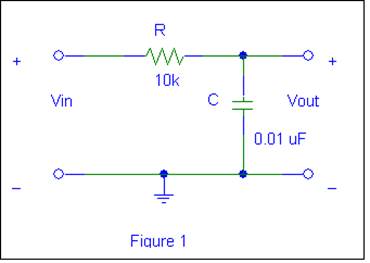
TIME DOMAIN RESPONSE Using Figure 1

Ø Drive Circuit 1 with a 2 volt peak-to-peak square wave (amplitude is not critical-look for minimal noise to set the amplitude) and observe the output. You will need to adjust the frequency of the square wave and oscilloscope sweep speed such that key attributes of the waveform are shown for a first-order response. The first order response equation is given by:

where τ is the time constant, τ = RC. A is the amplitude of v_in(t). You should be familiar with this equation and notation is from EE 2006.

Ø To measure the time constant, t, determine t_63% which is the time required for the output to reach 63% of its final value during a half-cycle of the input square wave. Does it equal the actual value of the RC product for your measured values of the resistors and capacitors you are using? Why or why not? You may need to change the horizontal time scale and vertical gain of the oscilloscope (and the amplitude of the input, if needed) to attain this measurement. Save key waveforms on flash drive. Measure and record the time constant t.

Ø Also, measure the rise time t_r and record. ( t_r = t_90% - t_10% = 2.2t). We will derive this in our initial laboratory discussion. Finally, compare the theoretical, experimental, and SPICE values of time constant and rise time.  Many of these measurements can be done by using soft key settings within the oscilloscope “MEASURE” menu. Fill in the following table. This is a good table to include in your lab report.

Parameter	Calculated	SPICE	Measured	Comments
Rise Time, tr
Time Constant, τ

Ø Now change the frequency of the input square wave from approximately 2 kHz to 30 kHz and adjust your amplitude appropriately to observe key waveform attributes so that you can observe that this circuit behaves as an analog passive integrator. That is over a limited range,

Ø Now apply a triangular wave to the input of the circuit. Note input and output waveforms, amplitudes and times. What output waveforms would you expect for integrating the square wave and triangular wave inputs? Do these measurements agree with the values and expected circuit time domain response you found using SPICE?

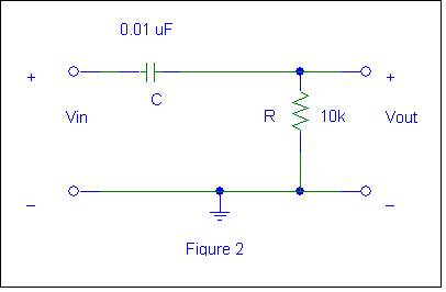
TIME DOMAIN RESPONSE Using Figure 2

Ø Drive Circuit 2 with a 2 volt peak-to-peak square wave (again amplitude is not critical) and observe the output. You will need to adjust the frequency of the square wave and oscilloscope sweep speed such that key attributes of the waveform are shown for a first-order response. The first order response equation is given by:

where the time constant τ = RC. A is the amplitude of v_in(t).

Ø To measure the time constant t, determine t_37% which is the time required for the output to reach 37% of “A” during a half cycle of the input. Does τ = RC for your measured values of the resistor and capacitor you are using? Why or why not? You may need to change the horizontal time scale and vertical gain of the oscilloscope (and the amplitude of the input, if needed) to attain this measurement. Save key waveforms on flash drive. Measure and record the time constant τ.

Ø Also, measure the fall time t_f and record. ( t_f = t_90% - t_10% = 2.2t). Finally, compare the theoretical, experimental, and SPICE values of time constant and rise time.  Many of these measurements can be done by using settings within the oscilloscope “MEASURE” menu. Fill in the following table. This is a good table to include in your lab report.

Parameter	Calculated	SPICE	Measured	Comments
Fall Time, tf
Time Constant, τ

Ø Now change the frequency of the input square wave from approximately 2 kHz to 30 kHz and adjust your amplitude appropriately to observe key waveform attributes so that you can observe that this circuit behaves as an analog passive differentiator. That is over a limited range, .

Ø Now apply a triangular wave to the input of the circuit. Note input and output waveforms, amplitudes and times. What output waveforms do you expect for differentiating the square wave and triangular wave inputs? Do these measurements agree with the values and expected circuit time domain response you found using SPICE?

Frequency Domain Response Using Figure 1 (Low-Pass Filter)

We will discuss the decibel (dB) in class on Wednesday, 18 January, and/or during the lab.

You will now demonstrate analog filters. Filters, whether analog or digital, are very important components in most electronic systems

The circuit in Figure 1 is also a basic single-pole analog, passive, low-pass filter (LPF). This LPF function can be observed by applying a constant-amplitude (i.e. 2 volt peak-to-peak amplitude input sinusoid and varying the frequency from 100 Hz to > 30 kHz.

Ø Measure, record and plot the voltage gain in dB and phase shift as a function of frequency (on a log scale). This is often called a Bode Plot. You may have seen similar plots for some of your audio stuff. Start at 100 Hz and end at a few tens of kHz. Measure the – 3 dB corner frequency of the filter, and the phase shift at that frequency. (Note that –3 dB corresponds to 70.7% of the low-frequency gain). Again, you can obtain phase directly from the “MEASURE” menu and visually verify by looking at the waveforms. Compare these measurements with theoretical and PSPICE values. Many of these measurements can be done by using soft key settings within the oscilloscope “MEASURE” menu.

Ø Compare your data to SPICE AC analysis plot.

FREQUENCY DOMAIN RESPONSE Of Figure 2 (High Pass Filter)

The circuit in Figure 2 is also a basic single-pole passive high-pass filter. To see this, observe the amplitude of the output as the frequency is varied from >30 kHz down to 100 Hz. You will need to use a 2 volt peak-to-peak constant-amplitude input sinusoid.

Ø Measure, record and plot the voltage gain in dB and phase shift as a function of frequency (on a log scale). This is often called a Bode Plot. Start at at a few tens of kH and end at 100 Hz. Measure the – 3 dB corner frequency of the filter, and the phase shift at that frequency. (Note that –3 dB corresponds to 70.7% of the high-frequency gain). Again, you can obtain phase directly from the “MEASURE” menu and visually verify by looking at the waveforms. Compare these measurements with theoretical and PSPICE values. Many of these measurements can be done by using soft key settings within the oscilloscope “MEASURE” menu.

Ø Compare your data to SPICE AC analysis plot.

Now for a little technically appropriate and politically correct humor from my collection of stuff. The first four are courtesy of Hewlett Packard/Agilent Instruments