Part 3: Patterns
Statistical analysis of sequences
Statistics of words
In this section we will consider the expected number of times a word (i.e. a given sequence of letters) occurs in a random sequence of letters. It is important to be precise about what we mean by "random sequence" - there are many different probabilistic models, and the best choice will depend on the context.
Here we will limit ourselves to the simplest model of random sequences, a Bernoulli model. It is what most people think of when they see the phrase "random sequence". Each letter in the sequence is independent from the others, and each has the same distribution. For example, the human genome is approximately 41% G+C and 59% A+T, so we could use the distribution p(\text{A}) =p(\text{T}) = 0.295, p(\text{C}) = p(\text{G}) = 0.205. The model is chosen for simplicity; real biological sequences often have additional structure. For instance in the human genome (and many others) the dinucleotide CG occurs much less often than the Bernoulli model would predict.
In the Bernoulli model it is easy to calculate the expected number of occurrences N(w) of a word w = (w_1, w_2, \ldots, w_k) in a sequence. First we note that probability of the word occuring at a particular position is
Then the expected number of occurrences in a sequence of length L is just
the number of places it is possible to have a sequence of length k times the probability of its occurrence at each position.
However, the variation of the number of occurrences is more subtle. It depends on the non-independence of the probabilities of the word appearing in two overlapping positions. In order to make this precise, we need a little more notation.
Let \epsilon_j(w) be a binary variable which is equal to 1 if the last j letters of w are the same as the first j letters of w; otherwise it is 0. For example, for the word w = \text{CCCGTGTCCC}, we have
and
Notice that \epsilon_9(w) = 1, since any word of length k has \epsilon_k(w) = 1.
The tendency for a word to overlap itself can be condensed into a single quantity, its autocorrelation coefficient \delta(w). In the Bernoulli model this is given by the sum of the probabilities of all the overlaps:
It is rather complicated to get an exact expression for the variance of N(w), but an excellent approximation when L is not too close to k is given by:
Example of word occurrence statistics
As an example of the above calculations we will look at the occurrence of some strings (words) in the human chromosome 22 sequence. This is one of the shortest human chromosomes, with about 36 million nucleotides on each strand. We will only work with one strand, although if you were interested in a biological motif you would probably want to check both strands (i.e. include the reverse complement).
First we will use the Biopython SeqIO module to load in the sequence, and a Counter object to count the occurrence of each letter:
from Bio import SeqIO
chr22 = SeqIO.parse('/Users/mh/bio/hs_ref_GRCh37.p10_chr22.fa','fasta')
from collections import Counter
letters = Counter()
for rec in chr22:
    for s in rec.seq:
        letters[s]+=1
freqs = {}
total = float(sum(letters.values()))
for w in letters:
    freqs[w] = letters[w]/total
Now the 'freqs' dictionary has the fraction of occurrence of each letter;
in this case p(\text{A})\approx p(\text{T}) \approx 0.26 and
p(\text{C})\approx p(\text{G}) \approx 0.24. Let us consider the occurrences of
ATTATA and CGCGCG. The autocorrelation coefficient of ATTATA is
0.26, since it has a single instance of overlap (\epsilon_1=1). The autocorrelation
coefficient \delta (\text{CGCGCG})\approx 0.06. The expected number and
standard deviation of these two words is
Now if we count the actual occurrences of these we find:
w1 = 'ATTATA'
w2 = 'CGCGCG'
w1counts = 0
w2counts = 0
chr22 = SeqIO.parse('/Users/mh/bio/hs_ref_GRCh37.p10_chr22.fa','fasta')
letters = Counter()
for rec in chr22:
    w1counts += rec.seq.count(w1)
    w2counts += rec.seq.count(w2)
print(w1counts)
print(w2counts)
    11042
    1041
The number of occurrences of ATTATA is within a standard deviation of
the expected value, so for that sequence the model seems to work well.
However the number of occurrences of CGCGCG is far below the expected
value - 65 standard deviations away! You do not need to compute a p-value
to know that the model hypotheses are invalid for the second word. In
this case, the main problem with our model is that the dinucleotide CG
is unusually rare in the human genome compared to what is expected from
a Bernoulli model (and more generally this dinucleotide is rare in most
Eukaryotes).
Exercise: Calculate the expected value and variance of the number of occurrences of the word AAAA and the word CGTA in a sequence of length 10^6, using the Bernoulli model with p(A) =p(T) = 0.375 and p(C) = p(G) = 0.125.
Exercise: For the same model as the previous problem, find a six letter word with the smallest variance possible.
Statistics of sequence alignment scores
One reason that the BLAST sequence alignment suite became overwhelmingly popular is its incorporation of a statistical model, the Karlin-Altschul statistical model. This model can be formally justified for alignments without gaps, and there is very strong empirical support for its extension to gapped alignments. In the Karlin-Altschul model, the probability that there are exactly k matches of a sequence of length n to a database of length m with scores at least S is given by the Poisson distribution
$$P(\text{k scores} \ge S) = \frac{e^{-E}E^k}{k!} $$ where the mean of this distribution is E, the expected number of matches with at least score S. The Karlin-Altschul theory suggests that
K is a parameter that is determined numerically, correcting for edge effects (important if the database consists of relatively short sequences) and other small discrepancies. \lambda is chosen to make \lambda S_{i,j} a log-odds scoring matrix (cf. Scoring Matrices section).
Since the probability of obtaining no scores \ge S is e^{-E}, the probability of getting one or more scores greater than or equal to S is
Since e^{-E} = 1 - E + E^2/2 + \ldots, once the E-value is small the probability of getting one or more scores greater than or equal to S becomes very close to E (since in that case 1-e^{-E} \approx E).
In comparing scores from different searches it is important to take into account the scoring matrix and database used. To normalize the score for different scoring matrices the bit score S' can be used:
$$S' = \frac{\lambda S - \ln K}{\ln 2} $$ and then the E-value can be written as E = m n 2^{-S'}. Since m is proportional to the size of the database, it is crucial when discussing an E-value to be clear about what database was used. In publishing results it is best to report this size as a particular database can grow over time (available from the 'search summary' tab in NCBI BLAST+).
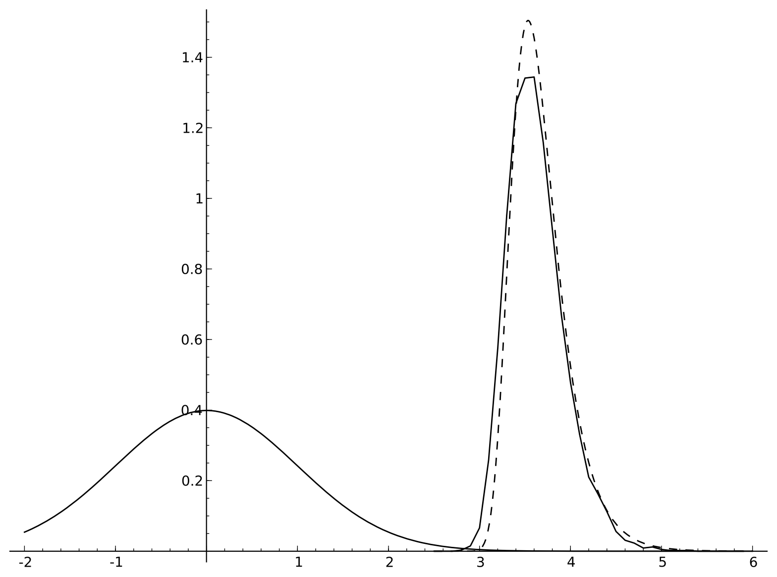
The probability distribution for BLAST is an example of an extreme value distribution, which arise when we look for extreme events. In this case, it is extremes of good alignments between sequences, but these distributions also appear in the study of floods, earthquakes, wildfires, financial markets, and sports. The normal (Gaussian) distribution is ubiquitous because of the central limit theorem, which says (roughly) that if you add together many values drawn from a single probability distribution, the resulting distribution will be close to the normal distribution. In a similar way, if we select extreme values from a distribution, the resulting extreme value distribution will be close to one of several possibilities, depending only on relatively coarse aspects of the tail of the original distribution. The most common case is when the original distribution has a normal-like tail, in which case the extreme value distribution will be a Gumbel distribution.
The Gumbel distribution has a cumulative distribution function $$G(x; \mu, \beta) = e^{-e^{-\frac{x - \mu}{\beta}}}. $$
In the case of alignment scores, we are interested in how significant we should consider a given maximum score. For this, we want the complement of the cumulative distribution function: 1 - G(x), since that measures the probability of having a score at least as high as x. We can rewrite this as:
to see that the Karlin-Altschul formula comes from an extreme value distribution with x = S, B = \lambda and A = K m' n'.
Below is a plot of a normal distribution, an empirically sampled extreme value distribution drawn from it, and a Gumbel distribution matching the empirical data's mean and variance. Because the cutoff score used was not that large (so the samples are not very extreme) the fit is not perfect.
Simple pattern recognition: Regular expressions and position-specific scoring matrices
Regular expressions
There are many situations in bioinformatics in which we wish to identify some sort of pattern in a sequence. Let us begin by considering a relatively well understood example: the \text{Cys}_2 \text{His}_2 zinc finger motif. This is a protein motif in which two cysteine and two histidine residues in a protein bind to a zinc ion, causing a finger-like loop in the protein. These fingers (usually more than one is present in a zinc finger protein) can bind to DNA, RNA, or sometimes other proteins.
Here are a few zinc finger motifs from some human proteins, with the critical cysteines and histidines shaded:
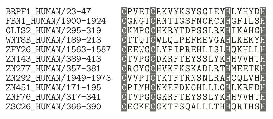
The pattern in this alignment is quite simple, and is well suited for what are called 'regular expressions' in computer science. We will not delve into all of the intricacies of regular expressions in general, but only on a subset that is most useful in bioinformatics. The notation for regular expressions in most programming languages can be intimidating at first, so we will concentrate on a more human-readable form developed for the database PROSITE. In the usual notation, the above zinc finger pattern could be written as
C.[4]C.[12]H.[5]H
which matches a C followed by any four letters, then a C, then any 12 letters followed by an H, any five letters, and finally another H. In the PROSITE notation this would be
C-x(4)-C-x(12)-H-x(5)-H
However, there are some closely related zinc fingers which are a little different:
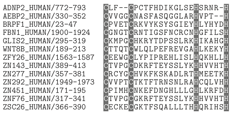
Now we need to allow some variability in the number of amino acids between the cysteines and histidines. For the above alignment, we might choose the regular expression
C-x(2,4)-C-x(12)-H-x(3,5)-H
which allows two to four residues between the cysteines and three to five residues between the histidines. The PROSITE regular expression PS00028 is built from 13,213 zinc finger motifs of this type, and they refined the pattern still further:
C-x(2,4)-C-x(3)-[LIVMFYWC]-x(8)-H-x(3,5)-H
This says that the four residues after the second cysteine must be one of the residues LIVMFYWC.
In some protein motifs, the residue at a particular position can be almost any amino acid, but some are incompatible with the motif's function. In these cases it is easier to describe the pattern by exclusion rather than inclusion. As an example, the alignment below shows some of the sequences in PROSITE's pattern PS00141, the active site motif for a group of aspartate proteases. The active site always contains an aspartate (D), which aids in cutting a peptide bond. The other residues in the motif show interesting constraints.
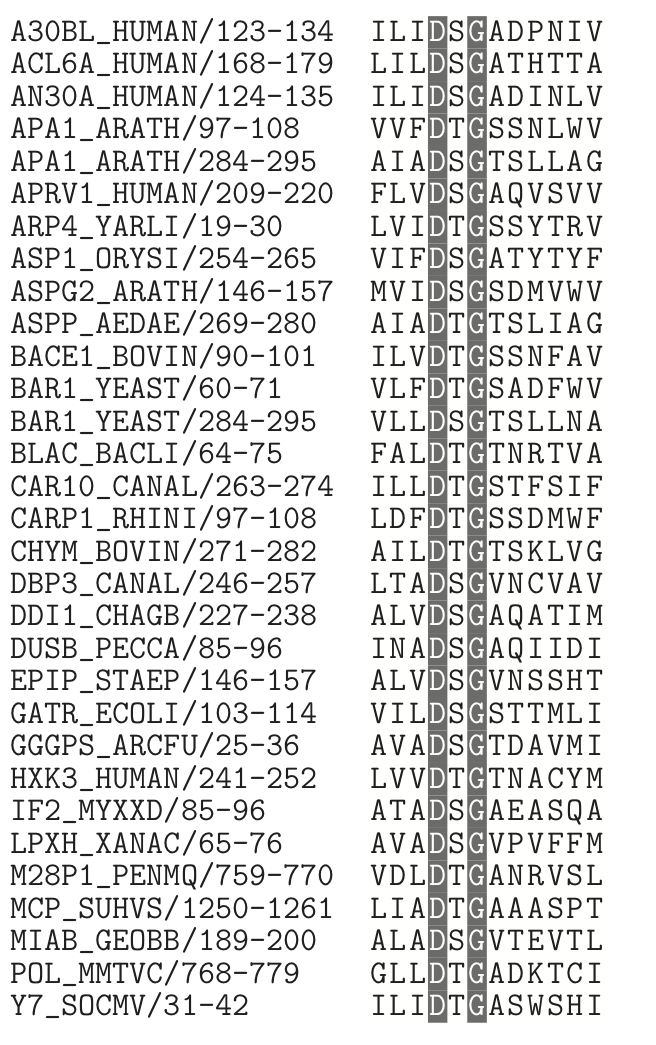
The regular expression for PS00141 is
[LIVMFGAC]-[LIVMTADN]-[LIVFSA]-D-[ST]-G-[STAV]-[STAPDENQ]
-{GQ}-[LIVMFSTNC]-{EGK}-[LIVMFGTA]
This means that in the ninth and eleventh positions the residues cannot be one of GQ or EGK, respectively.
Here is a summary of the PROSITE notation:
-
A set of amino acids in square brackets means that any one of those may be present in that position. So [CPW] would mean that a cysteine, proline, or tryptophan could be present in that position.
-
A hyphen simply seperates positions - they are otherwise meaningless. In regular expressions in programming languages, such redundant features are absent.
-
Curly brackets mean that anything but those residues (amino acids) can be present. So {P} would mean anything but a proline there.
-
An x means any residue is accepted.
-
Numbers in parentheses indicate multiple positions. So x(3) means any three residues. A pair of numbers gives a range, so C(3,4) means that there could be 3 to 4 cysteines there.
Exercises:
SAVGTGGMKTKIEAAEKA
ARHGSGGMVTKLMAARIA
TGISRGGMITKIRAAQRA
GDFATGGIVTKLIAADFL
NFKGVGGMRTKIKAAKIC
DPYSSGGMISKIEAGKIA
-
The above sequences are all from a family of glutamate-5 kinases. What are possible regular expressions that would include all these sequences? Which one would give the greatest specificity?
a [ADGNSTV]-x(2)-[GAS]-[RST]-G(2)-[IM]-x-[ST]-K-[LI]-x-A-[AG]-x(2)-[ALC]
b [ADGNST]-x(4)-G(2)-[IM]-x-[ST]-K-[LI]-x-A-[AG]-x(2)-[ALC]
c [ADGNST]-x(2)-[GAS]-x-G(2)-[IM]-x-[ST]-K-[LI]-x-A-[AG]-x(2)-[ALC]
d [ADGNST]-x(2)-[GAS]-x-G(2)-[IM]-x-[ST]-K-[LI]-x-A-[AG]-[EDKQR]-x-[ALC]
-
Construct a regular expression pattern for the following block of sequences. Try to make your expression specific and concise while matching all the listed sequences.
    GFNIVGYGCTTCLIG
    GARTEMPGCSLCMIG
    GFNLVGFGCTTCI-G
    GGMVLANACGPCIIG
    GFYLSGFGCTTCI-G
    GFEWRQSGCSMCL-A
    GVTLATPGCGPCL-G
    GALVCNPCCGPCLLG
- If the amino acids were independently and uniformly distributed (with frequencies of 1/20), approximately how many matches to your regular expression would you expect from a protein database with 3 million amino acids?
Position-specific scoring matrices
For some patterns regular expressions are too lacking in specificity because of the flexibility of composition within positions of the pattern. Consider the following hypothetical DNA motif alignment:
                                   ACTT
                                   ACCT
                                   ACAT
                                   AAGT
                                   AGGT
                                   ACGT
                                   ATGT
                                   GCGT
                                   CCGT
                                   TCGT
A regular expression would be pretty useless here because it would have to match all four letters in each of the first three columns:
x(3)-T
which is almost completely nonspecific. However, it seems that there are
more As in the first column, Cs in the second column, and Gs in
the third column. If we denote the proportion of the letter j in
column i by f_{i,j}, then for the above alignment we would have
| Letter | 1 | 2 | 3 | 4 |
|---|---|---|---|---|
| A | f_{1,A} = 0.7 | f_{2,A} = 0.1 | f_{3,A} = 0.1 | f_{4,A} = 0.0 |
| C | f_{1,C} = 0.1 | f_{2, C} = 0.7 | f_{3,C} = 0.1 | f_{4,C} = 0.0 |
| G | f_{1,G} = 0.1 | f_{2, G} = 0.1 | f_{3,G} = 0.7 | f_{4,G} = 0.0 |
| T | f_{1,T} = 0.1 | f_{2, T} = 0.1 | f_{3, T} = 0.1 | f_{4,T} = 1.0 |
We can use the distribution of letters in each column in the same way as in constructing protein scoring matrices if we choose a background distribution to compare them to. The simplest such background model for DNA would be to assume that each nucleotide is equally likely, p_A = p_C = p_G = p_T = \dfrac{1}{4}. Then the log-odds ratio for a letter j in the ith column would give a score S_{i,j} = \log \left ( \dfrac{f_{i,j}}{p_j} \right ). It is not too important which base we use for the logarithm, but the most common choice is to use logarithms with base 2, since then the scores can be interpreted in bits.
In our example, the consensus motif ACGT would give a total score of $$ S_{1,A} + S_{2,C} + S_{3, G} + S_{4, T} = 3 \log_2(\dfrac{0.7}{0.25}) + 2 \approx 6.46, $$ whereas the sequence CGAT would give a total score of
PSSMs can be visualized through sequence logos, in which each column is alloted a height equal to the relative entropy of the column's letter distribution (usually relative to the uniform distribution). Within each column, each letter is stacked inside with a height proportional to its frequency. A useful online tool with some examples is the "weblogo" site. Below is the sequence logo for the above example.
Hidden Markov Models
Introduction to HMMs
Hidden Markov Models (HMMs) are an extremely powerful class of probabilistic models with many applications in diverse fields such as speech recognition, bioinformatics, electrical engineering, and automated translation. Although the fundamental mathematical framework for HMMs was developed in the 1960s, their popularity exploded in the 1980s and 1990s. They are now one of the most widely used tools in bioinformatics for a variety of problems.
The backbone of any HMM is a Markov chain. A Markov chain is characterized by the property that the future behavior of a system is determined completely by its present state. More concretely, in our applications a discrete-time Markov chain consists of a set of states x_i, with probabilities t_{i,j} for the transition from state x_i to x_j. Consider the following toy example:
Example: Suppose we model the weather in a particular place in a very simple way, by classifying each day as either sunny (state S) or rainy (state R). In this location, the historical weather records show that sunny days followed by sunny days 80% of the time, while rainy days are followed by rainy days only 30% of the time. Lets denote the probability of it being sunny N days in the future by S_N and similarly the probability of it being rainy N days in the future by R_N. Then we can write the Markov model:
This can be repackaged as a vector-matrix equation, and then very powerful techniques from linear algebra can be used to analyze the system:
It is also very helpful to visualize a Markov chain model by drawing a diagram of the states and the weighted connections between them; for our simple weather model this would look like this:
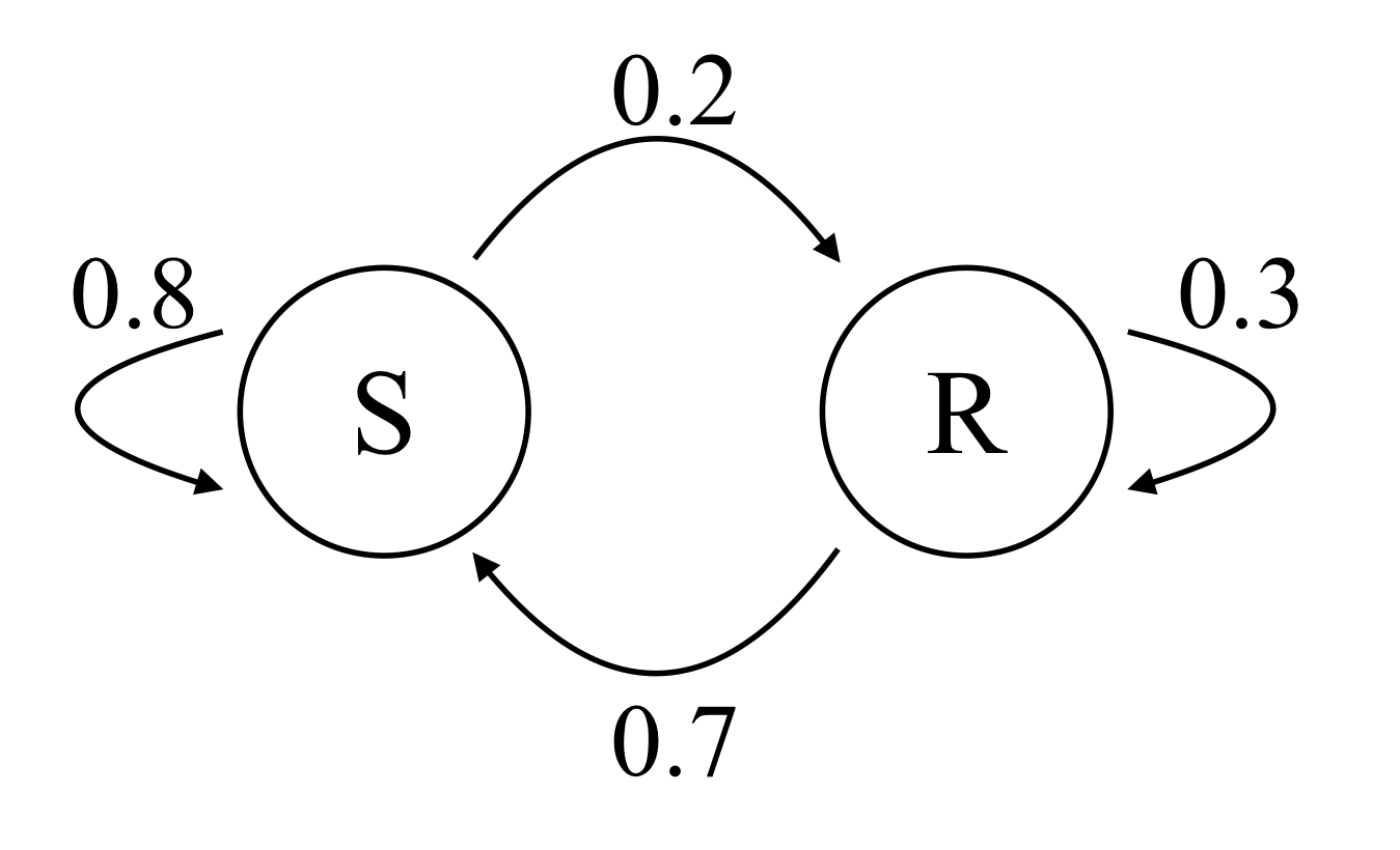
If every state can be reached (possibly in more than one step) from any other state, then the Markov chain is called irreducible. If a transition from some state to another can only occur in multiple of n steps, then the Markov chain is called periodic; if no pairs of states are periodic then the Markov is aperiodic. An irreducible, aperiodic Markov chain has the nice property that it will settle down into a unique stationary probability distribution. Finding this distribution amounts to the linear algebra problem of computing an eigenvector; for our weather model this problem looks like this:
where (S_{\infty}, R_{\infty} ) is the stationary distribution. In this case it turns out that (S_{\infty}, R_{\infty} ) \approx (0.78, 0.22), which means in the long run it will be sunny 78% of the time.
In a hidden Markov model (HMM), each state emits symbols from some alphabet with some probability distribution. We will denote the probability of the kth state to emit symbol x by P(x,k). Usually we are able to observe the emissions and not the underlying states.
Example: The two-bit grifter.
A con artist offers a superficially attractive deal: if you bet a dollar, he will flip a coin, and if it comes up heads you win 3 dollars; if it comes up tails he keeps the dollar. If you ask to see the coin he will show you a fair coin (having an equal chance to come up heads or tails). However, when playing this game he will sometimes switch to a loaded coin which comes up tails 90\% of the time. After using the loaded coin, he will switch back to the fair coin 1/3 of the time, but after using the fair coin he will switch to the loaded coin 2/3 of time. For the first coin toss, he will choose the fair or loaded coin with equal probability.
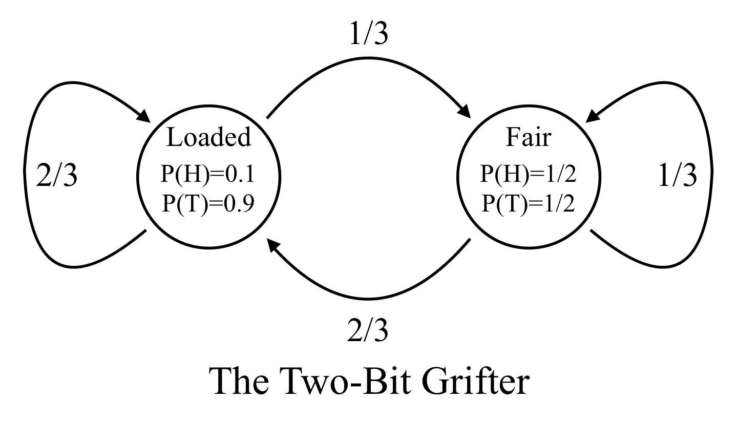
The underlying (hidden) states are use of the loaded (L) and fair (F) coin, and the observed emissions are heads (H) or tails (T).
The Viterbi algorithm
The Viterbi algorithm is another dynamic programming algorithm, used to compute the most probable sequence of hidden states in an HMM when given a sequence of emissions x = (x_1, x_2, \ldots, x_N). It requires knowing all of the parameters of the HMM.
Most HMMs have a special beginning state, which has transitions to other states i with initial probabilities \pi_i. We will denote the transition probabilities from state i to state j as a_{i,j}, and the set of all hidden states as Y. We denote the probability of state k for the tth emission by V(t,k). These dynamic programming quantities are initialized as $$V(1,k) = P(x_1, k)\pi_k. $$
Then the recursive relation for V_{t+1,k} in terms of the previous probabilities V(t,y) is
We also need to keep track of which y was used for the maximum with a 'pointer',
After computing these, we can traceback from the end by choosing a state with a maximal V(final,k) and then following the pointers:
Example: The two-bit grifter, continued
With the same parameters described previously, lets compute the most probably sequence of states (F=fair and L=loaded) for the two-bit grifter if we observe the coin flips H,T,T. For the first observation,
and
$$ V(1,L) = P(H,L) \pi_L = \frac{1}{10} \frac{1}{2} = \frac{1}{20} $$ and then
and for t=3:
The maximum of the V(3,y) is the loaded value (y=L), so the most probable reconstructed state sequence is F, L, L.
Forward, backward, and Baum-Welch algorithms
Instead of finding the most probable paths through an HMM, we can compute the most probable states (summed over all paths) for each emission in a sequence. This involves summing from a given state in both the forward and backward directions in the sequence, which is why the algorithm is called the forward-backward algorithm. This algorithm can be useful in itself, but its main utility is in fitting the parameters of an HMM using the Baum-Welch algorithm.
The forward part of the algorithm is similar to the Viterbi algorithm but with summations replacing maximizations. The quantity f(t,k) is the probability of observing (x_1, x_2, \ldots, x_t) given that the tth state is k. For the initial values we use the probability of the first emission weighted by the initial probability for that state:
and then continue recursively
The backward conditional probabilities b(t,k) are similar, but begin at t = N, the final emission. They are initialized to be 1:
and then are computed recursively for smaller t by
The quantities f and b can be used to compute the probability of being in state k at time t which we will denote by g(t,k):
In the Baum-Welch algorithm an HMM is iteratively modified using training data. For each sequence of observations, the forward and backward algorithms are used to estimate g(t,k), the probability of being in state k at time t, and the conditional probability of a transition from state k to state m at times t and t+1:
The parameters of the HMM - the initial state probabilities \pi, the state transition matrix a, and the emission probabilities P, are each updated to new values \tilde{\pi}, \tilde{a}, and \tilde{P} using g and c. Updating \pi is simplest:
To update a and P we average over the observation times:
where \chi_{x}(x_t) is an indicator function that is equal to 1 if x_t = x, and equal to 0 if x_t \neq x.
Usually this is repeated until the HMM parameters stabilize within some threshold. Note that the result is not guaranteed to be the best possible, it may just be close to a local maximum of likelihood in the space of parameters.
Example in Sage
Here we briefly illustrate implementing the 2-bit grifter example HMM in Sage. First we initialize the HMM with its state transition matrix probabilities, the emission probabilities, the initial state probabilities, and label the emissions:
transition_matrix = [[0.333, 0.667],[0.667, 0.333]]
emission_matrix = [[0.5,0.5],[0.1, 0.9]]
initial_probabilities = [0.5, 0.5]
emissions = ['H','T']
grifter_hmm = hmm.DiscreteHiddenMarkovModel(transition_matrix, emission_matrix,
    initial_probabilities, emission_symbols =emissions)
Next, we can examine the output of the HMM for a random sample; we print out the emissions and hidden states (using F for the fair coin, and L for the loaded):
from string import join
example_output = list(grifter_hmm.generate_sequence(20))
example_emissions = join(example_output[0], sep=' ')
def relabel_states(L):
    relabeled = [str(x).replace('0','F') for x in L]
    relabeled = ' '.join([x.replace('1','L') for x in relabeled])
    return relabeled
example_states = relabel_states(example_output[1])
print(example_emissions)
print(example_states)

    T H T T T T H T T H T H T H T T H T T T
    L F F L F L F L L F L F F L L L F L F L
In this example, the grifter is winning 70% of the time. If we did not know when he was using the loaded dice, we could try to reconstruct that with the Viterbi algorithm:
V = list(grifter_hmm.viterbi(example_output[0])[0])
V = relabel_states(V)
print(example_emissions)
print(example_states)
print(V)

    T H T T T T H T T H T H T H T T H T T T
    L F F L F L F L L F L F F L L L F L F L
    L F L L F L F L L F L F L F L L F L F L
The Viterbi estimated reconstructed states are on the last line. We can see it made three mistakes out of the 20 outputs - generally one cannot expect a perfect reconstruction unless the state emissions profiles are very different.
Now suppose a police surveillance camera has recorded 5000 coin flips by the grifter, but they do not know how often he switches coins or even how biased the loaded coin is. They attempt to use the Baum-Welch algorithm to correct a model in which they initially make reasonable guesses for the parameters:
transition_matrix = [[0.5, 0.5],[0.5, 0.5]]
emission_matrix = [[0.5,0.5],[0.05, 0.95]]
initial_probabilities = [0.5, 0.5]
emissions = ['H','T']
police_hmm = hmm.DiscreteHiddenMarkovModel(transition_matrix, emission_matrix, initial_probabilities, emission_symbols =emissions)
police_evidence = grifter_hmm.generate_sequence(5000)[0]
police_hmm.baum_welch(police_evidence, max_iter=1000)
    (-2990.1895582100938, 521)
The output of the Baum-Welch routine gives the log-likelihood of the sample under the updated HMM, and the number of iterations it took before converging. After this updating, the police's HMM has transition matrix:
which is much closer to what the grifter is doing than their initial guess.
The police HMM's updated emission matrix actually got worse, becoming:
To some extent this convergence to an incorrect model is an artifact of the simplicity of the emission possibilities, but it does show that there is no guarantee that the Baum-Welch algorithm will converge near a correct answer.
Exercises:
-
In the standard betting ("pass the line") in the game of Craps, you begin in the "come-out" state. Each round you roll two 6-sided dice, and total the result. In the come-out state, if you roll a 2, 3, or 12, you lose. If you roll a 7 or 11, you win. Otherwise, the number you roll becomes the "point" number (4,5,6,8,9, or 10). Once the point number is set, you continue rolling until you either roll the point again, in which case you win, or you roll 7, in which case you lose.
If we use the ordered list of states p = [\text{comeout}, \text{win}, \text{lose}, 4, 5, 6, 8, 9, 10], then we obtain a Markov chain with p_{i+1} = p_i T, where T is the transition matrix.
Complete the transition matrix below, and then draw the states and transitions as a graph. You do not have to label the edges with their weights, but do not include an edge if the transition value is zero.
T = \left(\begin{array}{rrrrrrrrr} 0 & \frac{2}{9} & \frac{1}{9} & & & & & & \\ 0 & 1 & 0 & 0 & 0 & 0 & 0 & 0 & 0 \\ 0 & & & & & & & & \\ 0 & \frac{1}{12} & \frac{1}{6} & \frac{3}{4} & 0 & 0 & 0 & 0 & 0 \\ 0 & & & \hspace{.2in} & \hspace{.2in} & \hspace{.2in} & \hspace{.2in} & \hspace{.2in} & \hspace{.2in} \\ 0 & \frac{5}{36} & \frac{1}{6} & 0 & 0 & \frac{25}{36} & 0 & 0 & 0 \\ 0 & \frac{5}{36} & \frac{1}{6} & 0 & 0 & 0 & \frac{25}{36} & 0 & 0 \\ 0 & \frac{1}{9} & \frac{1}{6} & 0 & 0 & 0 & 0 & \frac{13}{18} & 0 \\ 0 & \frac{1}{12} & \frac{1}{6} & 0 & 0 & 0 & 0 & 0 & \frac{3}{4} \end{array}\right) -
Compute the most probable path (for fair or loaded coins) for the two-bit grifter model for the observable sequence Tails, Heads, Heads, using the Viterbi model.
-
Suppose that the five amino acid sequences QRCCTGC, QCCGGCC, QCGCC, QCCCGCC, and QCCGC have the respective paths
m_1 i_1 m_2 m_3 m_4 m_5 d_6 m_7
m_1 m_2 m_3 m_4 m_5 m_6 m_7
m_1 m_2 d_3 d_4 m_5 m_6 m_7
m_1 m_2 m_3 m_4 m_5 m_6 m_7
m_1 m_2 m_3 d_4 m_5 d_6 m_7
through a protein HMM.
Write out the corresponding multiple sequence alignment.
-
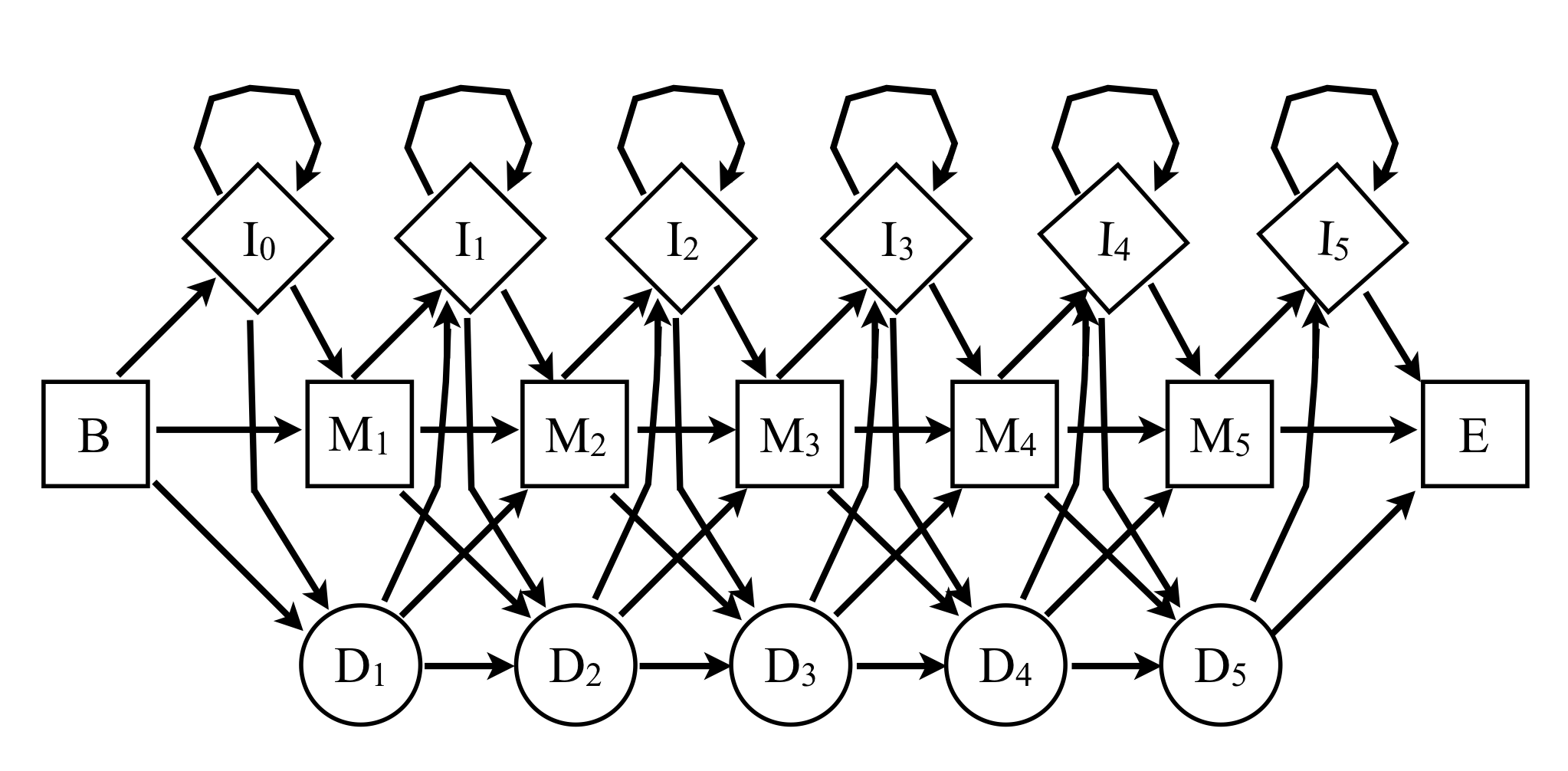
Consider a profile HMM as shown below, with the following properties:
-
The consensus sequence is QWERT; each match state emits the corresponding consensus letter with probability \dfrac{19}{20}, and any other amino acid letter with probability \dfrac{1}{380}.
-
The insertion states I_k emit each amino acid with probability \dfrac{1}{20}.
-
The B \rightarrow M_1 and M_i \rightarrow M_j transitions occur with probability \dfrac{7}{8}.
-
The M_i \rightarrow I_i and M_i \rightarrow D_{i+1} transitions occur with probability \dfrac{1}{16}.
-
The I_i \rightarrow I_i self-transitions occur with probability \dfrac{1}{4}.
-
The I_i \rightarrow M_{i+1} transitions occur with probability \dfrac{11}{16}, while Ii \rightarrow D(i+1) transitions occur with probability \dfrac{1}{16}.
-
Finally, the D_i \rightarrow D_{i+1} and D_i \rightarrow I_i transitions occur with probability \dfrac{1}{16}, while D_i \rightarrow M_{i+1} occurs with probability \dfrac{7}{8}.
-
What is the \log_2 likelihood of the most probable path of the consensus sequence in this model?
-
What is the alignment generated by the sequence QIWET, and what is its log likelihood? (You don't need to use the Viterbi method if you can guess the most probable path.)
-
How do the log likelihoods of the sequences AQWERT, AAQWERT, AAAQWERT, etc, compare to that of the consensus?
-
Artificial neural networks
Artificial neural networks (ANNs) are a class of machine learning algorithms. The name comes from biological inspiration - networks of interacting nodes. However, ANNs do not resemble modern models of actual neurons. The orginal name for the simplest and earliest types of ANNs was 'perceptron', perhaps a better name.
Early work on ANNs was limited by computational resources. In 1969 the simple perceptrons were mocked by Minsky and Papert, two influental researchers at MIT, and research in the area slowed. From about 1985 - 1995 they exploded in popularity, with considerable theoretical improvements. In the 21st century they have been largely overshadowed by other methods, but remain extremely useful for some problems.
After training on some input data, the final ANN is simply a function, mapping input vectors to output vectors. Usually the output is only one- or two-dimensional. For example, ANNs have been used to detect whether the beginning of a protein sequence is targeted to particular organelles such as the mitochondrion. In this case, the input would be very high in dimension, encoding the first 20 or so amino acids into a vector somehow, while the output would be a single number. If the output was above some threshold, then the sequence would be classified as mitochondrially targeted.
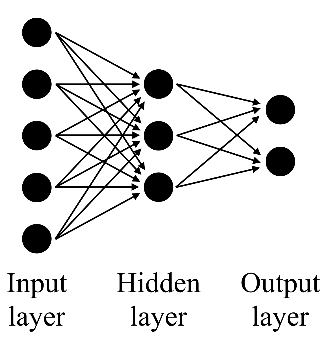
Each node in the network is a function, usually a composition of a univariate function and with a linear function of the inputs. That is, each of the inputs from other nodes are weighted to form a linear combination:
where the w_{ij} are the weights and the y_i are outputs of nodes which are inputs to node j. Then the output of node j is y_j = g(x_j). The form of the function g(x) is an important choice in the design of the ANN. A historically popular choice is
This function is sigmoidally increases from 0 to 1 over the real line. Unless the inputs are carefully normalized, this will not work well with most data unless a 'bias' parameter is introduced to the linear combination,
which can also be thought of as a constant input with weight \theta_j.
Backpropagation
The weights w_{ij} in the ANN need to be determined by training from data. Each datum is of the form (i_{q,1}, \ldots, i_{q,n}, o_{q,1}, \ldots, o_{q,m}) where the i_{q,j} are the inputs and o_{q,j} the desired outputs. Initially the weights are chosen randomly. The training seeks to minimize the total squared error
where the outer sum is over all the data q in the training set, and y_{q,k} is the output of the network given the training input.
The backpropagation algorithm is a gradient descent algorithm; we seek the minimum by altering the weights in the direction of the gradient of the error function. A parameter \eta must be chosen which determines how much we alter the weights at each step. For each weight we then update as follows:
The derivative \frac{\partial E}{\partial w_{ij}} can be calculated by using the chain rule:
Now we need to find the first partial derivative \frac{\partial E}{\partial x_j}. This is easiest when node j is in the output layer, so first consider that case. We will suppress the training set index q; the results would be summed over each of them.
The function g(x) = \frac{1}{1 + e^{-x}} is particularly convenient because its derivative can be written in terms of itself, namely
Once we have computed \frac{\partial E}{\partial x_j} for the output nodes, we can write the interior node weight derivatives in terms of them, so that our computations propagate from the output to the input layer.
Convolutional Deep ANNs
While potentially very powerful, ANNs require many design choices for best performance. Recently there has been much success with 'convolutional' ANNs which typically have the following properties compared with what we have described above:
-
They use a variety of output functions from their nodes, most often the rectified linear functions g(x;a) = \left \{ \begin{array}{c} 0 \text{ if } x \le 0 \\ ax \text{ if } x>0 \end{array} \right.
These are quite different from the logistic or 'soft step' function g(x) = \frac{1}{1 + e^{-x}} in that the output is unbounded.
-
They are called convolutional because of the structure and relations between the weights. Especially in the earlier layers of the network, sets of weights will be constrained to have the same value. This greatly lowers the dimension of the parameter space of weights, allowing the use of more nodes and layers. The layers are also not usually densely connected, but rather locally connected, with overlapping windows of connectivity.
-
The convolutional structure of the network makes it easier to parallelize the training of the weights. Powerful graphics processing units (GPUs) can be used for these parallel operations, making it possible to use many layers.
The convolutional structure is best suited for analyzing inputs that reflect a translation (or shift) invariance. For example, in image processing the local connections between early layers reflect the proximity of groups of pixels to each other. Similarly in analyzing audio signals, small connected windows can process high frequency components in the same way across the entire input.
Biological sequence analysis fortunately has this same shift invariance, making the convolutional ANNs very promising for bioinformatic applications.
RNA
The RNA world
One of the great mysteries of biology is how life arose. This question is still very much unanswered, but we do know enough to frame some promising hyptheses. The cell membrane, a lipid bilayer, can form spontaneously under the right conditions. Then the chemical environment inside the membrane can become quite different from the ambient solution, increasing the chance of reactions which might otherwise be too rare to occur. Amino acids can also form spontaneously under the right conditions. But one of the defining aspects of life, its self-replication, seems harder to imagine as a chance process. How did the ability of the cell to replicate DNA come about?
The most popular hypothesis explaining the origin of DNA replication is that it is RNA, not DNA, that first acquired a mechanism for self-replication.
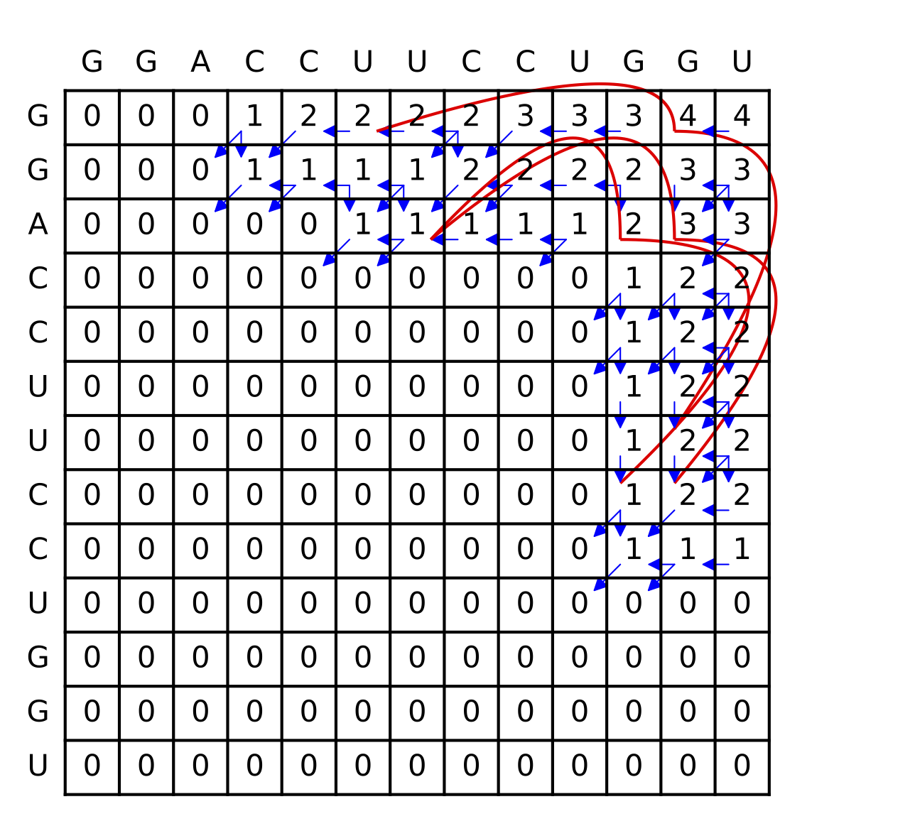
Nussinov pairing algorithm
In a pair of papers in 1978 and 1980, Ruth Nussinov and her coauthors proposed a dynamic programming algorithm for maximizing the number of base pairings in RNA.
In its simplest form, the Nussinov algorithm recursively computes the optimal pairing score \gamma(i,j) for the substrings x_i x_{i+1} \ldots x_j of a single string x = x_1 x_2 \ldots x_n.
The scores are initialized to disallow pairings between adjacent letters (since these are physically impossible for RNA molecules - they cannot bend 180 degrees between two adjacent nucleotides):
And the recursion formulae are:
Example
Below is the table of \gamma values for the RNA sequence GGACCUUCCUGGU. The traceback is shown in blue and red; for the last option in the recursion, each entry has two traceback paths (red).
Formal grammars
The Nussinov algorithm can be extended to a probabilistic model using the framework of stochastic grammars. A 'grammar' in this context is a set of symbols along with transformation rules that are applied on the symbols. If the transformation rules have an associated probability, then we have a stochastic grammar. The theory of formal grammars first arose in linguistics (introduced by Noam Chomsky in 1956), but their mathematical structure is useful in computer science, informatics, and related fields.
For a more thorough explanation of the use of stochastic grammars in bioinformatics, the book Biological Sequence Analysis: Probabilistic Models of Proteins and Nucleic Acids, by Richard Durbin, Sean R. Eddy, Anders Krogh, and Graeme Mitchison is highly recommended. The brief treatment here largely relies on their presentation.
In formal grammars there are two kinds of symbols, terminal and nonterminal. The nonterminal symbols do not occur in the final output of a grammatical process. A standard convention is to use capital letters for nonterminal symbols, and lowercase letters for terminal symbols. Often 'S' is used to indicate a unique initial (starting) symbol.
The simplest type of grammar is called a regular grammar. In a (right-)regular grammar there are only three types of allowed transformations. A nonterminal W can be transformed as follows:
-
W \rightarrow a where a is a terminal symbol.
-
W \rightarrow aX where a is a terminal symbol and X is a nonterminal symbol.
-
W \rightarrow \epsilon where \epsilon is the empty string.
A left-regular grammar is the same as above but with the second type of rule replaced by W \rightarrow Xa.
The regular grammars are equivalent to an object in computer science known as a finite state automaton, and to regular expressions. In bioinformatic applications, a stochastic regular grammars can be used to realize position-specific scoring matrices or Hidden Markov Models. The stochastic versions have probabilities for each transformation. The nonterminal symbols correspond to the hidden states in a HMM, and the terminal symbols to emissions.
A context-free grammar is more general than a regular grammar, including transformations of the form:
In order to formulate algorithms for working with context-free grammars, it is convenient to restrict the transformations to those in Chomsky Normal Form, in which only the allowed transformations are
The following stochastic context-free grammar (SCFG) can be used to implement a probabilistic version of the Nussinov algorithm:
Each possible transformation has a probability.
The equivalent of the Nussinov dynamic programming here is:
Initialization:
Recursion:
Exercise: Convert the grammar
into an equivalent Chomsky normal form by introducing new nonterminal symbols and transformations.
RNA-Seq and differential expression of genes
Here we describe a model of gene expression used by the program DESeq (Anders and Huber 2010). The number of reads from a gene i in a sample j is assumed to be drawn from a negative binomial distribution with mean \mu_{ij} and variance \sigma_{ij} (see section 16.1.3). The key assumption is then that the mean and variance have the form
where s_j is the coverage of reads for sample j, q_{i, j} is proportional to the expression of gene i in sample j, v is a smooth function, and \mu_{i,j} represents a background noise which is independent of depth of coverage.
Databases
Throughout this text we have used the word 'database' rather loosely, as a synonym for a collection of data. More specific definitions arise in the field of database management systems (DBMS), in which the data conforms to a formal model, and specialized software is used to manipulate this data.
The most well known example of a particular database framework is SQL (Structured Query Language). Python includes (as a module) an open source version of SQL called sqlite3. The wide support for sqlite3 makes it a good choice for storing fairly large collections of data that you might want to make application interfaces for (through a website for example).
Below is a short example of using sqlite3 in python, in which we make a single database table. The table has columns for the NCBI Taxonomy id of an organism, the scientific name of the organism, and the number of nucleotides records for that organism in NCBI's Nucleotide database. After creating a few rows, we update the values of one of the entries in the table.
import sqlite3
from string import join

connection = sqlite3.connect(DATA+"exampleTable.db")
crsr = connection.cursor()

# Create a table
crsr.execute('''CREATE TABLE life
             (taxid text PRIMARY KEY, name text, nuc int)''')
connection.commit()

# Insert a row of data
crsr.execute("INSERT INTO life VALUES ('9606', 'Homo sapiens', 27583474)")
crsr.execute("INSERT INTO life VALUES ('61851', 'Hoolock hoolock', 72)")
crsr.execute("INSERT INTO life VALUES ('34899', 'Petaurus breviceps', 862)")

# Save (commit) the changes
connection.commit()
crsr.execute("UPDATE life SET nuc=863 WHERE taxid='34899'")
connection.commit()

# Print out the table
crsr.execute("SELECT * FROM life")
ans= crsr.fetchall()
for i in ans:
    print(join([str(q) for q in i],sep='\t'))

    9606    Homo sapiens    27583474
    61851   Hoolock hoolock 72
    34899   Petaurus breviceps  863
Formal Ontologies
Ontology originally referred to a branch a philosophy concerned with the nature of existence and categories of being. Within informational sciences such as bioinformatics it now refers to a formalization of relationships between entities.
The Gene Ontology
GO, the Gene Ontology, is one of the most well developed and widely used ontologies in bioinformatics. Terms in GO are connected in a directed acyclic graph primarily through the 'is a' and 'part of' properties, although other relationships are supported. The relationships possible are themselves formalized in an ontology. Here is an example definition from the relation ontology:
[Typedef]
id: RO:0002589
name: results in catabolism of
def: "p results in catabolism of c if and only if p is a
catabolic process, and the execution of p results in c
being broken into smaller parts with energy being released." []
is_a: RO:0002586 ! results in breakdown of
Properties of compositions of relations are a kind of categorical mathematics. For properties such as 'part of' and 'is a', the study of their compositions is called mereology. In the Gene Ontology, an example of a mereological definition is that if A 'is a' B, and B is 'part of' C, then A is 'part of' C. This formalization is extremely difficult to get right, partly because our language is so ambiguous. For example, in everyday speech the ontological meaning of 'is a' can vary widely. In the phrase 'a dog is a mammal', the cat is a subtype of the mammal type. In the phrase 'Snoopy is a dog', Snoopy is a specific entity, an instantiation of the dog type. In the GO, only the former type of relationship is considered, and specific instances of types is avoided entirely.
Here are two term definitions from the GO definition file:
[Term]
id: GO:0008157
name: protein phosphatase 1 binding
namespace: molecular_function
def: "Interacting selectively and non-covalently with the enzyme
protein phosphatase 1." [GOC:jl]
is_a: GO:0019903 ! protein phosphatase binding

[Term]
id: GO:0005743
name: mitochondrial inner membrane
namespace: cellular_component
def: "The inner, i.e. lumen-facing, lipid bilayer of the mitochondrial
envelope. It is highly folded to form cristae." [GOC:ai]
synonym: "inner mitochondrial membrane" EXACT []
xref: NIF_Subcellular:sao1371347282
xref: Wikipedia:Inner_mitochondrial_membrane
is_a: GO:0019866 ! organelle inner membrane
is_a: GO:0031966 ! mitochondrial membrane
There are three components to the GO graph, with root terms 'biological process', 'cellular component', and 'molecular function'. These components are called namespaces.
The Sequence Ontology
The Sequence Ontology has a more narrow focus than the Gene Ontology, concerning itself only with biological sequences of DNA, RNA, and proteins. However, since these make up a large portion of all biological databases, it is an important particular area of concern. An example term definition from the SO is shown below:
[Term]
id: SO:0000118
name: transcript_with_translational_frameshift
def: "A transcript with a translational frameshift." [SO:xp]
synonym: "transcript with translational frameshift" EXACT []
is_a: SO:0000673 ! transcript
relationship: has_quality SO:0000887 ! translationally_frameshifted
Classes and Object Oriented Programming
The ideas involved in formal ontologies can be implemented in a variety of ways within informatics. Traditional databases are not very well suited to reflect the potential complexities of ontologies compared to class-based object oriented programming (OOP).
The idea of an object in computer programming became widespread in the 1960s with the creation of computer languages such as Simula and Smalltalk. An object in this context is an entity possessing an organized collection of subentities, which may be simple data types, functions, or complex sub-objects. In class-based languages such as C++ or Python, objects can belong to a hierarchy of classes. When this class hierarchy is not restricted to a tree structure (in CS parlance, the language supports multiple inheritance of classes), it is fairly simple to implement a formal ontology as classes of objects.
As an example of implementing a class, here is a simple class definition for dogs in Python:
class Dog:

    def __init__(self,name,breed):
        self.name = name
        self.breed = breed
        self.legs = 4

    def speak(self):
        return "Woof!"
The self argument of the internal functions refer to particular instances of the class (the objects).
This class can be instantiated as particular objects multiple times, for example:
Yippy = Dog('Yippy','Chihuahua')
Grif = Dog('Grif','German Shepard')
and these different instances store their own distinct names. If we need some instances to have more or different properties than others, we can create a subclass, e.g.:
class Chihuahua(Dog):

    def speak(self):
        return 'Yip!'
Now an instance of the Chihuahua will still be initialized as a Dog, and have the properties of a Dog, but the speak method will return 'Yip!' instead of 'Woof'.
For a more useful example, let us examine the 'Seq' class in the Biopython module. This class is used to encapsulate sequence information of various kinds, primarily RNA, DNA, and protein sequences. Some more specialized subclasses such as the 'CodonSeq' class inherit its properties.
Here is a brief illustration of the use of the Seq class, where its translate method is used. With the input:
from Bio.Seq import Seq
from Bio.Alphabet import IUPAC
rna_example = Seq("AUGGUCAUGCUAAGGGGC", IUPAC.unambiguous_rna)
rna_example.translate()
the output is a new Seq object containing the translation:
Seq('MVMLRG', IUPACProtein())