6. Eigenvectors and Eigenvalues - Introduction to ODEs and Linear Algebra

Gordon pic — Can you hear the shape of a drum?.

Eigenvectors and Eigenvalues

Definitions

We very often use a $n$ by $n$ matrix $A$ as a function on vectors, $f(x) = Ax$ , where the domain consists of $n$ -dimensional vectors ( $x$ ). The output of this function will be a vector that is stretched and rotated relative to the input $x$ . It turns out that it is very useful to look for vectors on which the function behaves in a simpler way, only stretching and not rotating the input.

Definition: A nonzero vector $v$ is an eigenvector of a square matrix $A$ with eigenvalue $\lambda$ if $A v = \lambda v$ .

It is important to remember that eigenvectors are defined to be nonzero. If you try to compute an eigenvector and you get the zero vector, something is wrong.

The eigenvalue $\lambda$ in the definition is a scalar (a number). So when acting on eigenvectors, the matrix multiplication reduces to just scalar multiplication. It is useful to allow the eigenvalues to be complex numbers, even for matrices with real entries.

The usefulness of eigenvectors and eigenvalues extends to the infinite-dimensional case, for example if we consider differential equations with solutions in some space of functions. In this context, eigenvectors are usually called eigenfunctions. For this text, the most important example of eigenfunctions are the exponentials, $e^{kt}$ , which are eigenfunctions of the differentiation operator: $\frac{d}{dt} e^{kt} = k e^{kt}$ .

Computing Eigenstuff

For large matrices the problem of finding eigenvalues and eigenvectors is not easy, and specialized numerical linear algebra algorithms are used for their computation. These are beyond the scope of this text. We will show how to compute them only for relatively small matrices.

We can rearrange the definition of an eigenvector-eigenvalue pair to get a linear homogeneous equation:

$A v = \lambda v \ \longleftrightarrow A v - \lambda v = 0$

$\longleftrightarrow A v - (\lambda I) v = 0$

$\longleftrightarrow (A - \lambda I) v = 0$

This square homogeneous linear system will only have a nonzero solution if the matrix $A - \lambda I$ is singular, which is equivalent to it having a determinant of zero. This gives us the characteristic equation of the matrix, whose solutions are the eigenvalues:

$\det(A - \lambda I) = 0$

Once we know the eigenvalues we can solve for the corresponding eigenvector to each eigenvalue.

Example: Computing Eigenvalues and Eigenvectors

Let's look at a small example, with the matrix

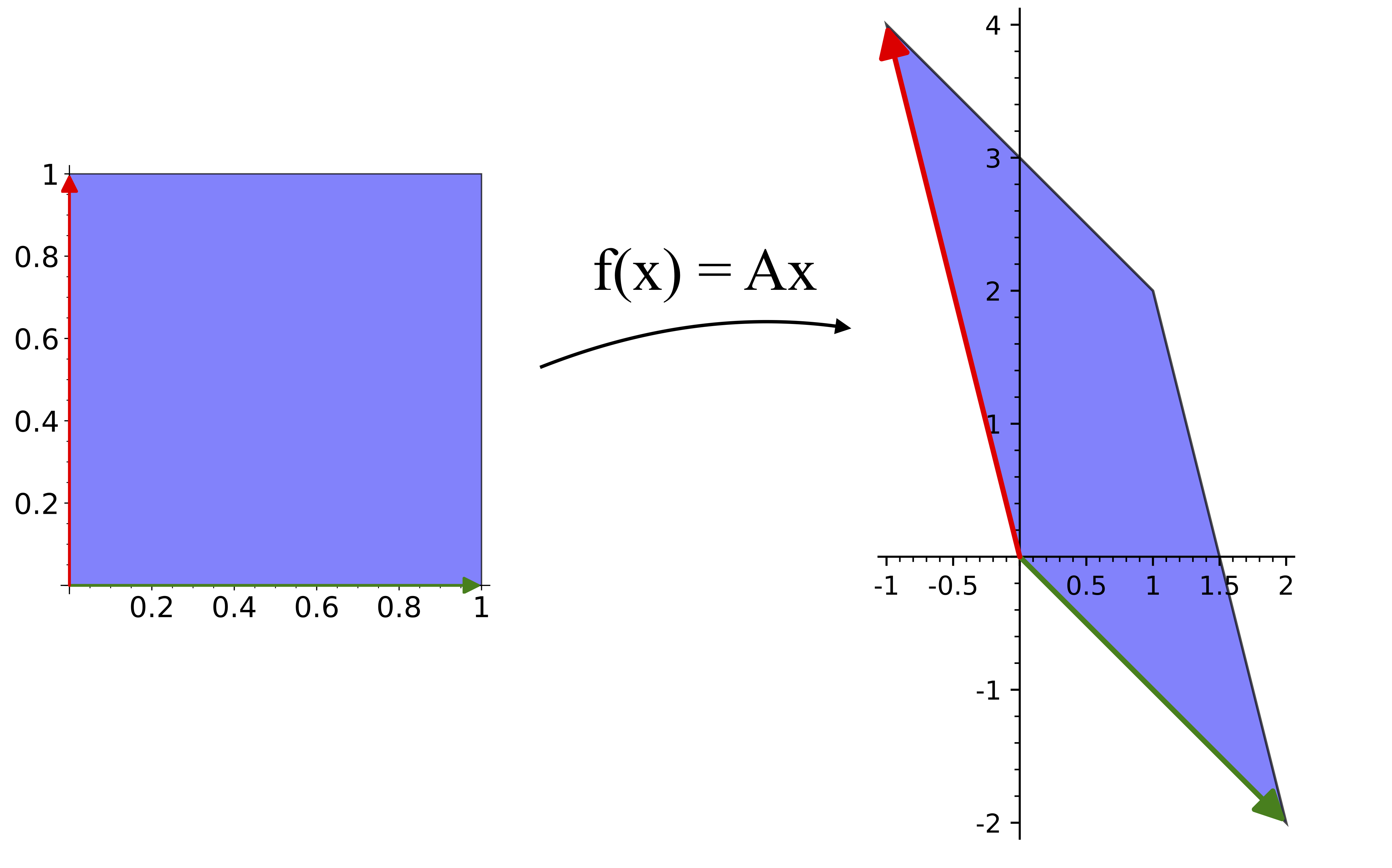
$A = \left(\begin{array}{rr} 2 & -1 \\ -2 & 4 \end{array}\right)$

matrix action — The effect of A on the unit square.

One way to think about the effect of a matrix is to consider its action on the unit coordinate vectors, $(1,0)$ and $(0,1)$ (transposed to be column vectors). These are sent to the first and second columns of $A$ , respectively, as shown in the figure. For this matrix, they are both stretched and rotated.

To find the eigenvalues we need the roots of the characteristic equation:

$0 = \det(A - \lambda I) = \det \left(\begin{array}{rr} 2 - \lambda & -1 \\ -2 & 4 - \lambda \end{array}\right)$

$= (2 - \lambda)(4 - \lambda) - (-1)(-2) = \lambda^2 - 6 \lambda + 6$

From the quadratic formula we find the two eigenvalues are $\lambda_1 = 3 - \sqrt{3}$ and $\lambda_2 = 3 + \sqrt{3}$ .

For each eigenvalue we need to find an eigenvector. Starting with $\lambda_1$ , we need a nonzero solution to the system:

$(A - (3 - \sqrt{3})I) v = \left(\begin{array}{rr} -1 + \sqrt{3} & -1 \\ -2 & 1 + \sqrt{3} \end{array}\right) v = 0$

To row-reduce the coefficient matrix lets begin by multiplying the top row by the top right entry's conjugate, $-1 - \sqrt{3}$ , gives us

$\left(\begin{array}{cc} -1 + \sqrt{3} & -1 \\ -2 & 1 + \sqrt{3} \end{array}\right) \ \longrightarrow \left(\begin{array}{rr} -2 & 1 + \sqrt{3} \\ -2 & 1 + \sqrt{3} \end{array}\right)$

and now we see that we can eliminate one row entirely. After subtracting row 1 from from 2 and then dividing row 1 by $-2$ , we get the RREF

$\left(\begin{array}{cc} 1 & -\frac{1}{2} - \frac{\sqrt{3}}{2} \\ 0 & 0 \end{array}\right)$

If our eigenvector has components $a$ and $b$ , then we must have $a + b(-\frac{1}{2} - \frac{\sqrt{3}}{2}) = 0$ . We can choose $b=1$ , and then $a = \frac{1}{2} + \frac{\sqrt{3}}{2}$ . So our first eigenvector is

$v_1 = \left(\begin{array}{c} \frac{1}{2} + \frac{\sqrt{3}}{2} \\ 1 \end{array}\right)$

In a similar way, the other eigenvector $\lambda_2 = 3 + \sqrt{3}$ gives us the system

$(A - (3 + \sqrt{3})I) v = \left(\begin{array}{rr} -1 - \sqrt{3} & -1 \\ -2 & 1 - \sqrt{3} \end{array}\right) v = 0$

and the coefficient matrix is row-reducible to

$\left(\begin{array}{cc} 1 & -\frac{1}{2} + \frac{\sqrt{3}}{2} \\ 0 & 0 \end{array}\right)$

with eigenvector

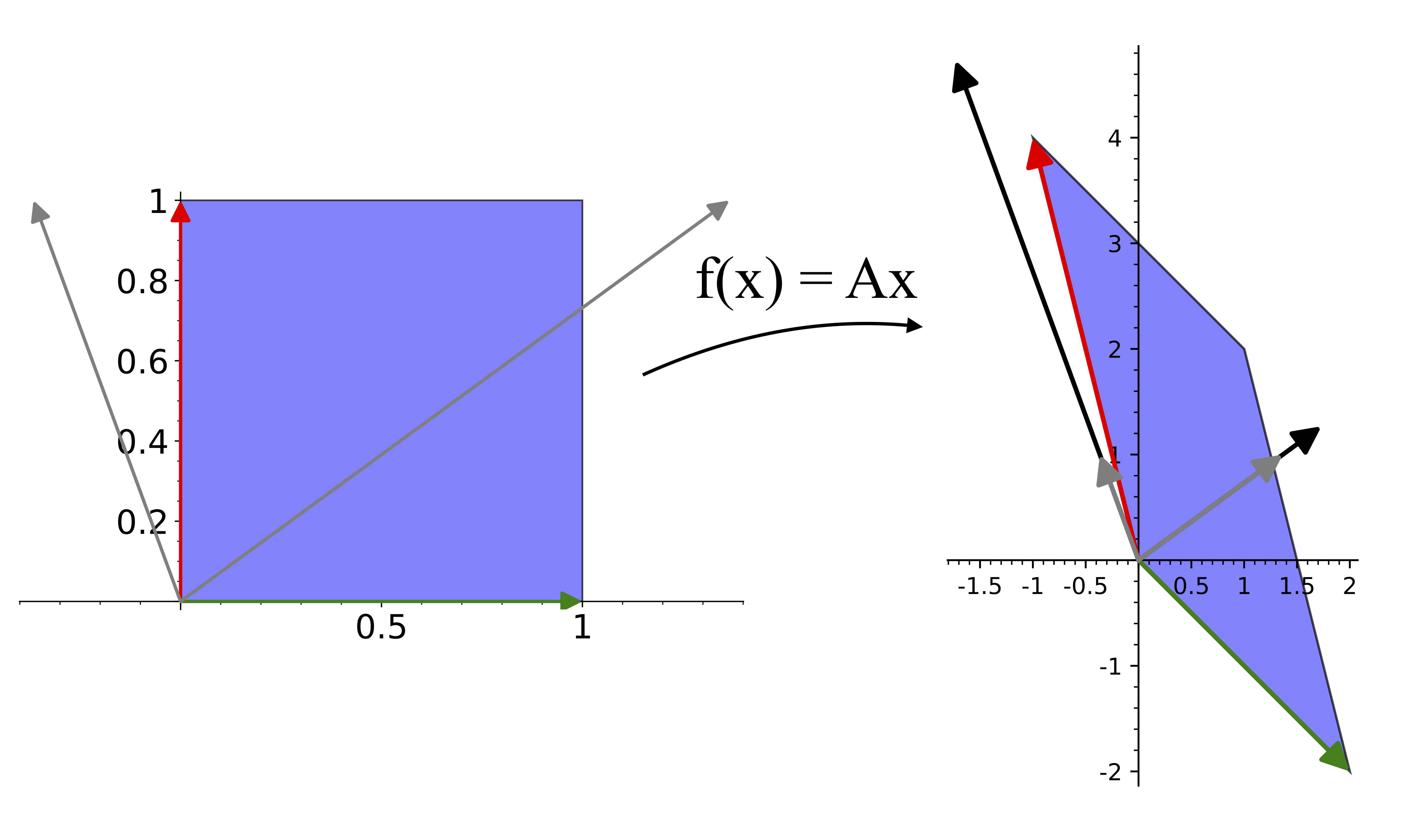
$v_2 = \left(\begin{array}{c} \frac{1}{2} - \frac{\sqrt{3}}{2} \\ 1 \end{array}\right)$

The figure below shows the action of $A$ on the eigenvectors (in gray, with $Av$ in black). Both eigenvalues are larger than 1, so both eigenvectors are stretched out by $A$ .

matrix action with eigenvectors — The effect of A on the unit square with its eigenvectors.

Diagonalization and Similarity

If a $n$ by $n$ matrix $A$ has $n$ linearly independent eigenvectors, we can use them to transform $A$ into a diagonal form. If $P$ is a $n$ by $n$ matrix whose columns are linearly independent eigenvectors of $A$ , then

$A P = P D \text{ or equivalently } A = P D P^{-1}$

where $D$ is a diagonal matrix whose diagonal entries are the eigenvalues of $A$ ,

$D = \left ( \begin{array}{cccc} \lambda_1 & 0 & \ldots & 0 \\ 0 & \lambda_2 & \ldots & 0 \\ \vdots & \vdots & \ddots & \vdots \\ 0 & 0 &\ldots & \lambda_n \end{array} \right )$

This allows the relatively easy computation of arbitrary powers of $A$ since

$A^n = (P D P^{-1})^n = (P D P^{-1} P D P^{-1} \ldots P D P^{-1}) = P D^n P^{-1}$

and

$D^n = \left ( \begin{array}{cccc} \lambda_1^n & 0 & \ldots & 0 \\ 0 & \lambda_2^n & \ldots & 0 \\ \vdots & \vdots & \ddots & \vdots \\ 0 & 0 &\ldots & \lambda_n^n \end{array} \right )$

Example: power computation through diagonalization

$A = \left( \begin{array}{ll} 4 & -3 \\ 2 & -1 \end{array} \right)$

let's first compute the eigenvalues and eigenvectors of $A$ . For the eigenvalues, the characteristic equations is

$\det(A - \lambda I) = (4 - \lambda)(-1 - \lambda) + 6 = \lambda^2 - 3 \lambda + 2$

$= (\lambda - 1)(\lambda - 2) = 0$

so the eigenvalues of $A$ are $\lambda_1 = 1$ and $\lambda_2 = 2$ . Now we find the eigenvectors by computing the kernel of $A - \lambda I$ for each eigenvalue $\lambda$ :

$A - I = \left( \begin{array}{ll} 3 & -3 \\ 2 & -2 \end{array} \right) \rightarrow \left( \begin{array}{ll} 1 & -1 \\ 0 & 0 \end{array} \right)$

has kernel vectors $\left( \begin{array}{l} c \\ c \end{array} \right)$ for any $c$ , so we can choose $v_1 = \left( \begin{array}{l} 1 \\ 1 \end{array} \right)$ .

Similarly

$A - 2I = \left( \begin{array}{ll} 2 & -3 \\ 2 & -3 \end{array} \right) \rightarrow \left( \begin{array}{ll} 1 & -3/2 \\ 0 & 0 \end{array} \right)$

has kernel vectors $\left( \begin{array}{l} 3c \\ 2c \end{array} \right)$ for any $c$ , and we can choose $v_2 = \left( \begin{array}{l} 3 \\ 2 \end{array} \right)$ .

The matrix $P$ is then

$P = \left ( v_1 | \ v_2 \right ) = \left( \begin{array}{ll} 1 & 3 \\ 1 & 2 \end{array} \right)$

with inverse

$P^{-1} = \left( \begin{array}{rr} -2 & 3 \\ 1 & -1 \end{array} \right)$

and now we can compute

$A^{10} = P D^{10} P^{-1} = \left( \begin{array}{ll} 1 & 2 \\ 1 & 3 \end{array} \right) \left( \begin{array}{ll} 1^{10} & 0 \\ 0 & 2^{10} \end{array} \right) \left( \begin{array}{rr} -2 & 3 \\ 1 & -1 \end{array} \right)$

$= \left( \begin{array}{ll} 1 & 2 \\ 1 & 3 \end{array} \right) \left(\begin{array}{rr} 2 & -3 \\ 2^{10} & -2^{10} \end{array}\right) = \left(\begin{array}{rr} 3 \cdot 2^{10}-2& 3(1-2^{10})\\ 2^{11}-2 & -2^{11}+3 \end{array}\right) = \left(\begin{array}{rr} 3070 & -3069 \\ 2046 & -2045 \end{array}\right)$

Matrix Similarity

We have seen that a square matrix $A$ is diagonalizable if $A = P D P^{-1}$ for some diagonal matrix $D$ . More generally, if $A$ , $B$ , and $C$ are all $n$ by $n$ matrices, then $A$ is similar to $B$ if there is a $C$ such that

$A = C B C^{-1}$

The matrix $C$ acts as a change of coordinates (or change of basis), so if $A$ and $B$ are similar it means they represent the same transformation in different coordinates. This means that as matrices they have many things in common, including their trace and determinant.

Exercises:

Compute the eigenvectors and eigenvalues of the matrix

$A =\left( \begin{array}{rr} 2 & 1 \\ 1 & 2 \end{array}\right)$
Compute the inverse $P^{-1}$ of the matrix $P = (v_1 | v_2)$ where the $v_i$ are linearly independent eigenvectors of $A$ .
Use the fact that $A^n = P D^n P^{-1}$ , where $D$ is a diagonal matrix, to compute $A^{10}$ .

Complex eigenvalues and eigenvectors

Matrices with real entries can have complex eigenvalues and eigenvectors. This will be important in the next chapter, where we study systems of linear differential equations through the eigenvalues and eigenvectors of their coefficient matrices.

If the matrix has real entries, any complex eigenvalues and eigenvectors will appear in complex-conjugate pairs. Knowing this is helpful, since it means as soon as you compute half of the pair you can determine the other half simply by taking the complex conjugate.

Example: eigenstuff of rotation matrices

In the plane, the matrix

$A = \left(\begin{array}{rr} \cos(\theta) & -\sin(\theta) \\ \sin(\theta) & \cos(\theta) \end{array}\right)$

applied from the left ( $Ax$ ) on a vector $x$ will rotate it counter-clockwise by the angle $\theta$ . Lets compute its eigenvalues and eigenvectors.

The characteristic equation is

$\det(A - \lambda I) = \det \left(\begin{array}{rr} \cos(\theta) - \lambda & -\sin(\theta) \\ \sin(\theta) & \cos(\theta)- \lambda \end{array}\right) = \lambda^2 - 2 \cos(\theta) \lambda + 1 = 0$

where we have simplified terms using the identity $\cos(\theta)^2 + \sin(\theta)^2 = 1$ . The roots of the polynomial are

$\lambda = \cos(\theta) \pm i \sin(\theta) = e^{\pm i \theta}$

The eigenvector for $\lambda = \cos(\theta) + i \sin(\theta)$ must be in the kernel of

$A - (\cos(\theta) + i \sin(\theta))I = \left(\begin{array}{rr} -i \sin(\theta) & -\sin(\theta) \\ \sin(\theta) & -i \sin(\theta) \end{array}\right) = \sin(\theta) \left(\begin{array}{rr} -i & -1 \\ 1 & -i \end{array}\right)$

After dividing by $\sin(\theta)$ (lets assume it is not zero), we can add $i$ times the bottom row to the top and see that the rref will be $\left(\begin{array}{rr} 1 & -i \\ 0 & 0 \end{array}\right)$

and we can choose the eigenvector to be

$v_1 = \left( \begin{array}{r} i \\ 1 \end{array} \right)$

The other eigenvector, with eigenvalue $\cos(\theta) - i \sin(\theta) = e^{-it}$ is the complex conjugate of this,

$v_2 = \left( \begin{array}{r} -i \\ 1 \end{array}\right)$

Eigenvector deficiency

It is possible for square matrices to be deficient in eigenvectors, in the sense that there may not be a complete basis of eigenvectors. Such matrices are not diagonalizable, but we can get as close as possible to a diagonalized form. The most common choice of this almost-diagonal form is called the Jordan normal form, named after the engineer and mathematician Camille Jordan. Completely characterizing the Jordan normal form for all matrices is beyond the scope of this text; we will only consider what happens in the 2 by 2 and 3 by 3 matrix cases.

The 2 by 2 case is relatively simple - there are only 2 possible types of Jordan normal forms. If a 2 by 2 matrix $A$ has eigenvalues $\lambda_1$ and $\lambda_2$ , then

$P^{-1} A P = J_A = \left( \begin{array}{rr} \lambda_1 & 0 \\ 0 & \lambda_2 \end{array}\right) \ \text{ or } \ \left( \begin{array}{rr} \lambda_1 & 1 \\ 0 & \lambda_1 \end{array}\right)$

The second form is only possible when $\lambda_1 = \lambda_2$ . In this case, the similarity matrix $P$ is not a matrix of eigenvectors - only the first column of $P$ is an eigenvector.

Example: A 2 by 2 eigenvector deficient Jordan normal form

We will find a similarity matrix to put the matrix

$A = \left( \begin{array}{cc} 4 & 1 \\ -4 & 0 \end{array} \right)$

into its Jordan normal form.

First we compute the eigenvalues of $A$ with the characteristic equation

$\det (A - \lambda I) = \det \left( \begin{array}{cc} 4 - \lambda & 1 \\ -4 & - \lambda \end{array} \right) = \lambda^2 - 4 \lambda + 4 = 0$

which has a double root $\lambda_{1,2} = 2$ .

The eigenvectors of $A$ with eigenvalue $2$ will be in the kernel of $A - 2I$ . If we compute the reduced row echelon form of $A - 2I$ we get

$A - 2 I = \left( \begin{array}{cc} 2 & 1 \\ -4 & -2 \end{array} \right) \longrightarrow \left( \begin{array}{cc} 1 & 1/2 \\ 0 & 0 \end{array} \right)$

This only has a 1-dimensional kernel, spanned by the eigenvector $v = (1,-2)^T$ . So this matrix is not diagonalizable.

To get the other column of our similarity matrix we want a vector that is not an eigenvector, but which becomes one after it is multiplied by $A - 2$ . Equivalently, we want a vector in the kernel of $(A-2)^2$ that is not an eigenvector. Since

$(A-2)^2 = \left( \begin{array}{cc} 2 & 1 \\ -4 & -2 \end{array} \right) \left( \begin{array}{cc} 2 & 1 \\ -4 & -2 \end{array} \right) = \left( \begin{array}{cc} 0 & 0 \\ 0 & 0 \end{array} \right)$

we can pick any nonzero vector that is not a multiple of $v$ . Lets pick $w = (1,0)^T$ for simplicity. The image of this under multiplication by $A-2$ is

$(A - 2)w = \left( \begin{array}{cc} 2 & 1 \\ -4 & -2 \end{array} \right) \left( \begin{array}{c} 1 \\ 0 \end{array} \right) = \left( \begin{array}{c} 2 \\ -4 \end{array} \right) = 2v$

For a similarity matrix we can now choose

$P = (2v | w) = \left( \begin{array}{cc} 2 & 1 \\ -4 & 0 \end{array} \right)$

and we can verify

$P^{-1} A P = \left( \begin{array}{cc} 0 & -1/4 \\ 1 & 1/2 \end{array} \right) \left( \begin{array}{cc} 4 & 1 \\ -4 & 0 \end{array} \right) \left( \begin{array}{cc} 2 & 1 \\ -4 & 0 \end{array} \right) = \left( \begin{array}{cc} 0 & -1/4 \\ 1 & 1/2 \end{array} \right) \left( \begin{array}{cc} 4 & 4 \\ -8 & -4 \end{array} \right) = \left( \begin{array}{cc} 2 & 1 \\ 0 & 2 \end{array} \right)$

For a 3 by 3 matrix there are three types of Jordan normal form. If the eigenvalues are $\lambda_1$ , $\lambda_2$ , and $\lambda_3$ , the possible Jordan normal forms (up to reordering our choices of eigenvalues) are

$\left( \begin{array}{ccc} \lambda_1 & 0 & 0 \\ 0 & \lambda_2 & 0 \\ 0 & 0 & \lambda_3 \end{array}\right) , \ \left( \begin{array}{ccc} \lambda_1 & 1 & 0 \\ 0 & \lambda_1 & 0 \\ 0 & 0 & \lambda_3 \end{array}\right) , \ \left( \begin{array}{ccc} \lambda_1 & 1 & 0 \\ 0 & \lambda_1 & 1 \\ 0 & 0 & \lambda_1 \end{array}\right)$

Higher dimensional eigenspaces

We choose eigenvectors as a representative of the subspace they span; the subspace (an eigenline) is a more fundamental object but it is convenient to have a concrete element of it for computations. Sometimes a higher dimensional space is uniformly scaled by the same eigenvector, and in this case we have even more freedom than usual in choosing the representatives. Lets look at an example.

Example of higher dimensional eigenspaces

Find a set of linearly independent eigenvectors for the projection matrix

$P = \left(\begin{array}{rrrr} 0 & \frac{1}{2} & -1 & 1 \\ 0 & 1 & 0 & 0 \\ 0 & -1 & 1 & -1 \\ 0 & -1 & 0 & 0 \end{array}\right)$

(The definition of a projection matrix is that $P^2 = P$ ; i.e. once a vector has been projected, repeating the application of the projection does nothing further.)

The characteristic equation is

$\det (P - \lambda I) = (\lambda - 1)^2 \lambda^2 = 0$

so the eigenvalues are $0$ , $0$ , $1$ , and $1$ .

For the eigenvalue $0$ , we compute the reduced row echelon form of the matrix $P$ itself,

$rref(P) = \left(\begin{array}{rrrr} 0 & 1 & 0 & 0 \\ 0 & 0 & 1 & -1 \\ 0 & 0 & 0 & 0 \\ 0 & 0 & 0 & 0 \end{array}\right)$

From this we see that any vector $v = \left(\begin{array}{r} a \\ b \\ c \\ d \end{array} \right)$ in the kernel of $P$ needs to have $b=0$ and $c - d=0$ . There are two free variables, $a$ and $d$ . This means we can choose two linearly independent eigenvectors. A systematic way to do this is to choose one with $a=1$ and $d=0$ , and the other with the complementary choice $a=0$ and $d=1$ :

$v_1 = \left(\begin{array}{r} 1 \\ 0 \\ 0 \\ 0 \end{array} \right) \ , \ v_2 = \left(\begin{array}{r} 0 \\ 0 \\ 1 \\ 1 \end{array} \right)$

Similarly, for the multiple eigenvalue of $1$ we need to compute the rref of $P - I$ , which is

$rref(P - I) = \left(\begin{array}{rrrr} 1 & 0 & 1 & -\frac{1}{2} \\ 0 & 1 & 0 & 1 \\ 0 & 0 & 0 & 0 \\ 0 & 0 & 0 & 0 \end{array}\right)$

The components of any eigenvectors with eigenvalue $1$ must satisfy $a+c-d/2=0$ and $b+d=0$ . The non-pivot variables $c$ and $d$ are free. Again we can make the two linearly independent choices $c=1$ , $d=0$ and $c=0$ , $d=1$ to get

$v_3 = \left(\begin{array}{r} -1 \\ 0 \\ 1 \\ 0 \end{array} \right) \ , \ v_4 = \left(\begin{array}{r} 1/2 \\ -1 \\ 0 \\ 1 \end{array} \right)$

Additional Exercises

Find a matrix $P$ such that $P^{-1}AP = D$ , where $D$ is a diagonal matrix, for the matrix $A$ below if such a $P$ exists, or explain why it does not exist.

$A = \left(\begin{array}{rrr} 0 & 1 & 0 \\ -1 & 2 & 0 \\ -1 & 1 & 1 \end{array}\right)$
Find a matrix $P$ such that $P^{-1}AP = D$ , where $D$ is a diagonal matrix, for the matrix $A$ below if such a $P$ exists, or explain why it does not exist.

$A = \left(\begin{array}{rrrr} 1 & 0 & 0 & 1\\ 0 & 1 & 0 & 1 \\ 0 & 0 & 1 & 1 \\ 0 & 0 & 0 & 2 \end{array}\right)$
Show that if $A$ is invertible and $\lambda$ is an eigenvalue of $A$ , then $1/\lambda$ is an eigenvalue of $A^{-1}$ . Are the eigenvectors the same?
By computing the eigenvalues and eigenvectors of

$A = \left(\begin{array}{rr} 3 & -2 \\ 1 & 0 \end{array}\right)$

find a matrix $P$ such that $P^{-1}AP = D$ where $D$ is a diagonal matrix. Use this diagonalization to compute $A^6$ .

Notes

Notes: (Local storage in a cookie)

License

This work (text, mathematical images, and javascript applets) is licensed under a Creative Commons Attribution-NonCommercial-ShareAlike 4.0 International License. Biographical images are from Wikipedia and have their own (similar) licenses.