Systems of differential equations
Homogeneous Linear ODE systems with the eigenstuff method
In this section we will look at how to use eigenvalues and eigenvectors to solve a homogeneous linear system of ODEs:
where x is a n-dimensional vector and A is a n by n (square) matrix.
The main idea is to diagonalize A as much as possible by using the eigenvectors of A as a basis. Unfortunately not every matrix A has a complete basis of n linearly independent eigenvectors. For now we will assume that our A does have such a basis \{ v_1, v_2, \ldots, v_n \}, with
If we put these eigenvectors into a matrix P = (v_1 | v_2 |\ldots|v_n) as columns, then if x = P y (or equivalently y = P^{-1} x) our differential equation becomes
where D is the diagonal matrix of eigenvalues with diagonal entries D_{i,i} = \lambda_i. We can multiply this ODE on the left by P^{-1} to get
which nicely splits into n independent scalar ODES:
These have solutions
The answer to our original problem is x = P y, which in terms of the eigenvectors and eigenvalues is
If all of the eigenvalues \lambda_i are real, then this is the general solution to the system. If some of the eigenvalues are complex we need to work a little bit more to extract the real part of the solution.
If we have a complex conjugate pair of eigenvalues \lambda = A + iB, \bar{\lambda} = A - iB and associated eigenvectors v and \bar{v}, there is a 2-parameter component of the solution of the form
where Re and Im are the real and imaginary parts of the complex vector.
Another way to look at this method is that we are matching up the eigenfunctions of the differentiation operator (the exponential functions) with the eigenvectors of the matrix.
Example
Let's look at a relatively simple example of the above procedure:
Because the coefficient matrix is symmetric (A_{i,j} = A_{j,i}) it will have a complete set of eigenvalues with real eigenvalues. We use the characteristic equation to find the eigenvalues:
Using the quadratic formula we get \lambda_1, \lambda_2 = 3 \pm \sqrt{2}.
For each \lambda we need to find a non-zero solution v_i of (A - \lambda_i I) v_i = 0 by row-reducing each matrix (A - \lambda_i I). For \lambda_1 = 3 + \sqrt{2} we get
and we can choose
Similarly for \lambda_2 = 3 - \sqrt{2} we can choose
and the general solution to the differential equation is
Exercises:
-
Solve the initial value problem x_1' = 6 x_1 - 7 x_2, x_2' = x_1 - 2 x_2, x_1(0) = 4, x_2(0) = 1.
-
For which values of a, b, and c is the determinant of the matrix below equal to zero?
\left(\begin{array}{ccc} 1& a & a \\ b & b & b \\ c & c & 1 \end{array}\right) -
Matrices A and B shown below each represent a rotation in three dimensional space. Matrix A rotates 45 degrees counterclockwise around the z axis, and matrix B rotates 45 degrees around the x axis.
A = \left(\begin{array}{ccc} \frac{\sqrt{2} }{2} & -\frac{\sqrt{2} }{2} & 0 \\ \frac{\sqrt{2} }{2} & \frac{\sqrt{2} }{2} & 0 \\ 0 & 0 & 1 \end{array}\right), \ \ \ \ B = \left(\begin{array}{ccc} 1 & 0 & 0 \\ 0 & \frac{\sqrt{2} }{2} & -\frac{\sqrt{2} }{2} \\ 0 & \frac{\sqrt{2} }{2} & \frac{\sqrt{2} }{2} \end{array}\right)The combination of rotating with matrix A followed by B is represented by C = BA. The matrix C can be thought of as representing a single rotation around some axis.
a. Find that axis of rotation by computing the eigenvector of C with eigenvalue 1.
b. Find a basis for the subspace of vectors perpendicular to the axis from part (a). (A column vector v is perpendicular to another vector w if w^T v= 0.)
Initial value problems and sketching in the plane
Planar (2-D) systems of differential equations are nice because we can visualize their behavior pretty easily, and they are also important because higher-dimensional systems can often be at least partially analyzed in terms of planar components with the eigenvalue/eigenvector method.
In this section we will consider a couple of linear initial value problems in the plane, and look at their trajectories.
The first example has real eigenvalues and eigenvectors, which makes it a little easier to understand and to sketch.
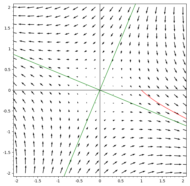
Example: Saddle point
Find the solution to the initial value problem
First we compute the eigenvalues of the coefficient matrix from the characteristic equation:
So \lambda_{1,2} = \pm \sqrt{2}. Now we need an eigenvector for each eigenvalue.
For \lambda_{1} = \sqrt{2} the eigenvector needs to be in the kernel (or nullspace) of A - \sqrt{2} I, which we row-reduce:
and we can choose v_1 = \left(\begin{array}{c} -1 - \sqrt{2} \\ 1 \end{array}\right) (any other nonzero multiple would also work). Similarly for \lambda_2 = -\sqrt{2}, we get
and we can choose v_2 = \left(\begin{array}{c} -1 + \sqrt{2} \\ 1 \end{array}\right)
The general solution to the system is
Substituting in the initial condition x(0) = (1,0)^T we have the linear algebraic system
We can row-reduce the augmented coefficient matrix, or use simple substitution to find that C_1 = -\frac{1}{2 \sqrt{2}}, C_2 = \frac{1}{2 \sqrt{2}} and so
Below is a plot of the solution in red, and with the span of each eigenvector shown in green. The solution approaches the span of the eigenvector v_1, since that component grows exponentially with t, and the other component shrinks exponentially.
The next example has complex eigenvalues, which means the solution will involve sine and cosine functions as well as exponentials - the solution will spiral around the origin in such cases. If the real part of the eigenvalues are negative, it will spiral in, and if the real parts are positive it will spiral out. If the real parts are zero (purely imaginary eigenvalues) then the solutions will consist of concentric elliptical trajectories.
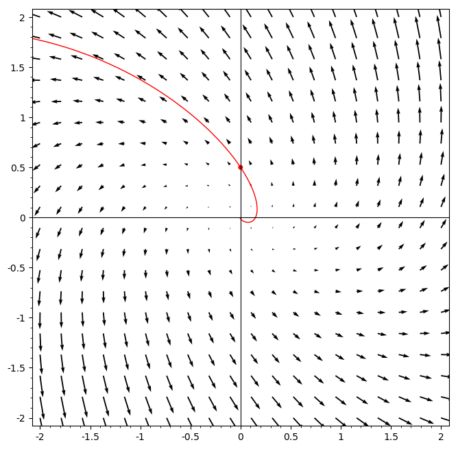
Example: Unstable spiral
Find the solution to the initial value problem
The characteristic equation of this coefficient matrix is
which has the complex roots \lambda_{1,2} = 2 \pm i \sqrt{3}.
For complex eigenvalues we only need to compute one eigenvector. For \lambda_1 = 2 + i \sqrt{3}, we have
and we can choose
The general solution is then
Using the initial condition x_1(0) = 0 and x_2(0) = 1/2, we have the equations
so C_2 = \frac{1}{2\sqrt{3}}, and the solution is
The positive real part of the eigenvalues results in the expansive e^{2t} factor in the solution, causing the solution to exponentially spiral out, in this case counter-clockwise. The plot below shows the slope field and the particular solution of this problem (in red), with the starting point at t=0 indicated by a dot.
Exercises
- Solve the initial value problem
Euler's method for systems.
The fundamental idea of Euler's method for numerical approximation of ODE solutions does not change when we apply it in the setting of first-order systems: we extend a solution to a new point using a tangent-line approximation. The only change is that the slope function, and the solution itself, are vector-valued. Let us look at an example.
Example
Approximate the solution to the initial value problem
at t=4 using four steps of Euler's method.
Since we are going from t=0 to t=4 in four steps, our stepsize is h = 1. Since we are already using subscripts for vector components let us call the approximate solutions a_0, a_1, etc. We begin at a_0 = x(0) = (1, 0)^T, and compute a_1:
The next three steps are very similar. At each step we only need the values from the previous one:
Our relatively large step size has resulted in a very unstable approximation, which diverges sharply from the true solution on the last step, where a_{4,0} = 1340 but the true solution is approximately x_1(4) \approx 0.57.
Exercises
-
Suppose a rocket from Earth is launched by a railgun from a height h=0, and after its initial burn it is at an altitude of h = 5 km with a velocity of 10 km/s straight up.
-
If we use an approximation of a constant gravitational acceleration g = 0.0098 km/s{}^2 (and no air resistance), how high will the rocket be after 100 seconds?
-
A more realistic approximation would use the Newtonian gravitational acceleration of the Earth:
\frac{d^2h}{dt^2} = - \frac{g R^2}{(h+R)^2}where R = 6378 km is the radius of the Earth. Write this as a first-order system with variables h and v = \frac{dh}{dt}, and use Euler's method to estimate the height of the rocket after 100 seconds with two steps. Is this new estimate an over-estimate or under-estimate?
-
Multi-compartment models
Previously we considered compartment (tank) problems which could be solved as a series of single-variable linear ODEs. For most compartment problems however the compartments (or tanks) have enough interactions that they must be analyzed as a system. If the model is linear, we can solve these systems with the eigenvalue/eignevector method.
Example: 3 tank problem
Consider three connected tanks of equal volume V_i=10 liters, with 3 L/minute pumped from tank 1 into tank 2, and 3 L/minute pumped from tank 2 to tank 3, and finally 3 L/minute pumped from tank 3 into tank 1. If initially tank 1 has 2 grams of salt dissolved in it, and the other tanks have pure water, find the amount of salt in each tank as a function of time. We can assume that the compartments are well-stirred at all times.
Let us denote the amount of salt in each tank by x_1, x_2, and x_3. The initial conditions are x_1(0) = 2, x_2(0) = 0, and x_3(0) = 0. The differential equations for these amounts are
or in vector-matrix form
To proceed we need the eigenvalues of the coefficient matrix, so we need to factor the characteristic equation
We see that \lambda_1 = 0 is an eigenvalue and the other two roots can be computed from the quadratic formula:
To find the eigenvector with eigenvalue 0 we need to row reduce the matrix A:
The simplest choice of the eigenvector v_1 for which A v_1 = 0 would be
For the complex eigenvalues we only need to compute one of the eigenvectors; the other will be the complex-conjugate of the first. For \lambda_2 = - \frac{9}{20} + i \frac{3 \sqrt{3}}{20} we need to row reduce A - \lambda_2 I:
and we can choose the eigenvector v_2 to be
To write the real general solution we need to extract the real and imaginary parts of v_2 e^{\lambda_2 t}:
These real and imaginary parts can be used as independent real components, giving us the general solution:
We can now substitute the initial conditions, which gives us
The augmented coefficient matrix for this system is
which can be row-reduced to
and finally we can see that C_1 = \frac{2}{3}, C_2 = -\frac{2}{3}, and C_3 = -\frac{2\sqrt{3}}{3}. The final solution simplifies a little to:
The exponential e^{\left(-\frac{9}{20} t\right)} will become very small as t increases, and the solution will approach the completely mixed state with x_1 = x_2 = x_3 = \frac{2}{3}.
A common source of confusion on this type of problem is that the initial conditions do not directly affect the differential equations.
Exercises
-
Consider three well-stirred tanks, each containing 1 liter. r liters of fluid per minute is sent from tank 1 to 2, from tank 2 to tank 1, from tank 2 to tank 3, and from tank 3 to tank 2. Initially tank 1 is filled with pure water, tank 2 is filled with brine at a concentration of 2 grams of salt per liter, and tank 3 is filled with brine at a concentration of 4 grams per liter.
a. Write down the differential equations and initial conditions for the amount of salt in each tank (x_1, x_2, and x_3).
b. Solve the differential equations.
c. Find a value of r so that the concentration of salt in tank 3 is three times that of tank 1 at time t=1 minute.
Eigenvector deficiency example: the Moog ladder filter
Sometimes the coefficient matrix of a linear system of ODEs does not have a basis of eigenvectors. These systems are rare in the sense that a small random perturbation of the matrix entries will almost always alter the eigenvalues to be distinct, and the perturbed matrix will have a basis of eigenvectors. However they do arise in some applications; here we will illustrate one way to solve such systems using the example of the (linearized) four-stage Moog ladder filter.
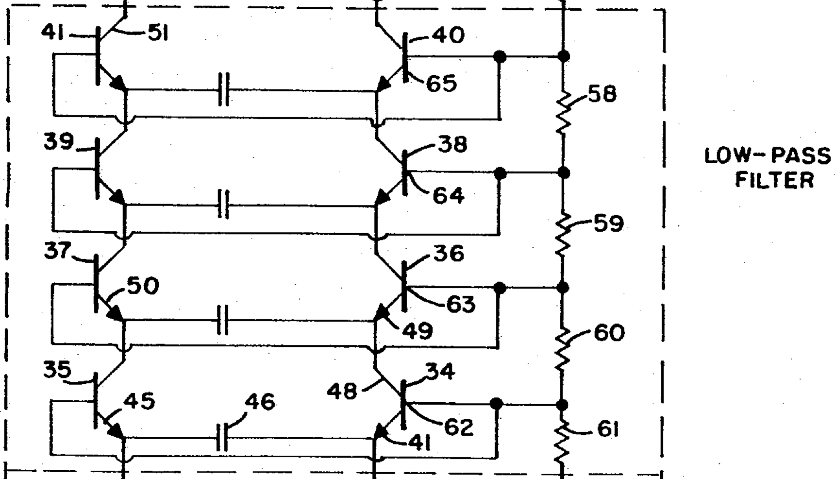
The linearized equations for the voltages y_i in each stage, with input x(t), cutoff parameter \alpha, and resonance parameter r are
or in matrix form
When the resonance parameter r is zero, the coefficient matrix A has only one eigenvalue \lambda equal to -\alpha. If we try to find eigenvectors for this eigenvalue, we see there is only one linearly independent vector in the kernel of A + \alpha I:
The eigenvector must be a multiple of v = (0,0,0,1)^T. This means the homogeneous solution has a component C_4 v e^{-\alpha t}. It must have three additional linearly independent components.
In general we can solve this kind of problem by introducing a cascade of so-called generalized eigenvectors, which can be found by studying the kernels of (A - \lambda I)^m for different powers of m. To describe this systematically is beyond the scope of this text; we'll just look at what happens in this particular case.
We can note that the first equation of the homogeneous system is independent of the others, with y_1' = -\alpha y_1. The solution to that is y_1 = C_1 e^{-\alpha t}. Then the next equation would be
which is a first order linear equation with solution
We can continue down the ladder solving 1st order linear equations to get
and
In vector form, we can write this solution as
and we can see the last column is the eigenvector solution we originally knew.
Second order mass-spring systems
For many applications, including interacting mechanical, electrical, and chemical systems, the damping (friction) terms are relatively small and do not strongly affect the natural modes of vibration of the system. In these cases the differential equations have the form
where x is a vector and A is a constant square matrix. With some experience with square matrices it is natural to guess that the solution may be decomposed into pieces related to the eigenvectors of A, so suppose that x is of the form f(t) v_i where v_i is an eigenvector of A. Substituting that into the ODE system yields
and we see that we need to have f'' = \lambda_i f, where \lambda_i is the eigenvalue for v_i. For oscillating systems we usually have non-positive eigenvalues \lambda_i \le 0, which it is convenient to write as positive frequencies \lambda_i = - w_i^2, or w_i = \sqrt{-\lambda_i}. For w_i \ge 0 the solution to
is
and this means if we have a complete set of eigenvectors v_i we can write the general solution as
In the special case that \lambda = 0, we get a pair of solutions v_i (C_{2i} + C_{2i+1} t). This means the system is invariant under translations, and choosing C_0 and C_1 amounts to choosing a coordinate system.
The animation below shows an example with two equal masses. The top motion is a weighted combination of the two normal modes of oscillation, which are shown below it.
Example: Mass-Spring System
Suppose that one mass (m_1 = 2) is connected to a rigid wall with a spring of stiffness k_1 = 100, and a second mass (m_2 = 1) is connected to the first mass with a spring of stiffness k_2 = 50. The differential equations for the deviations of each mass from its equilibrium position are:
After substituting in our values for m_1, m_2, k_1, and k_2, we can divide by the masses and put this into the matrix-vector form:
The characteristic equation of the coefficient matrix is
which has solutions \lambda_1 = -25 and \lambda_2 = -100.
The eigenvectors are in the kernel (nullspace) of A - \lambda_i I for each eigenvalue. For \lambda_1 we have
and one choice of eigenvector is v_1 = \left(\begin{array}{c} 1 \\ 2 \end{array}\right).
For \lambda_2 = -100 we have
and a simple choice of eigenvector is v_1 = \left(\begin{array}{c} 1 \\ -1 \end{array}\right).
The frequencies for these eigenvalues are w_1 = \sqrt{-\lambda_1} = 5 and w_2 \sqrt{-\lambda_2} = 10, so the solution is
The two natural modes of oscillation corresponding to these eigenvector/eigenvalue pairs are a slower (w_1 = 5) in-phase oscillation of the two masses moving in the same direction, and a faster (w_2=10) oscillation in which the two masses are moving in opposing directions.
Exercises
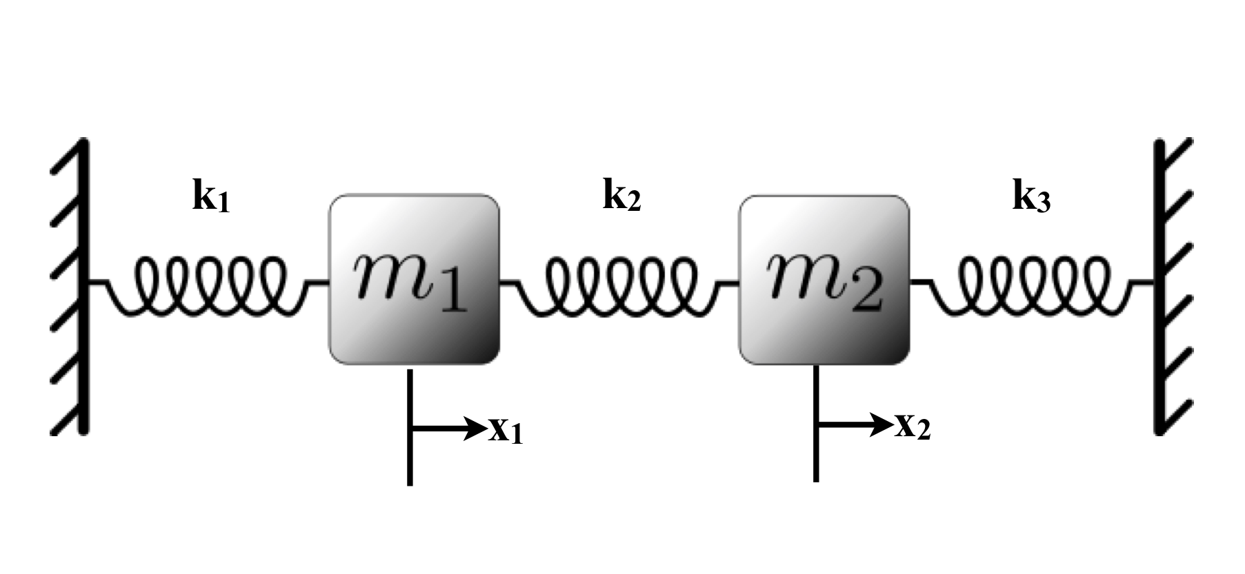
- Consider two blocks of mass m_1 = m_2 = 1 connected by springs to each other and to walls as shown below. The displacement of the masses from their equilibrium positions are denoted by x_1 and x_2. The stiffness of the three springs are k_1 = 4, k_2=6, and k_3=4. Compute the natural frequencies and describe the normal modes of oscillation.
Extended example (lab project): Earthquake-building resonances
This example/exercise is intended for exploration with a computer algebra system such as Sage - it is too difficult to complete by hand.
The goal is to model the response of a moderately tall building (seven stories) to vibrations induced by an earthquake. We model the building as seven coupled masses, each of mass m, with a linear spring coupling between adjacent floors with spring constant k.
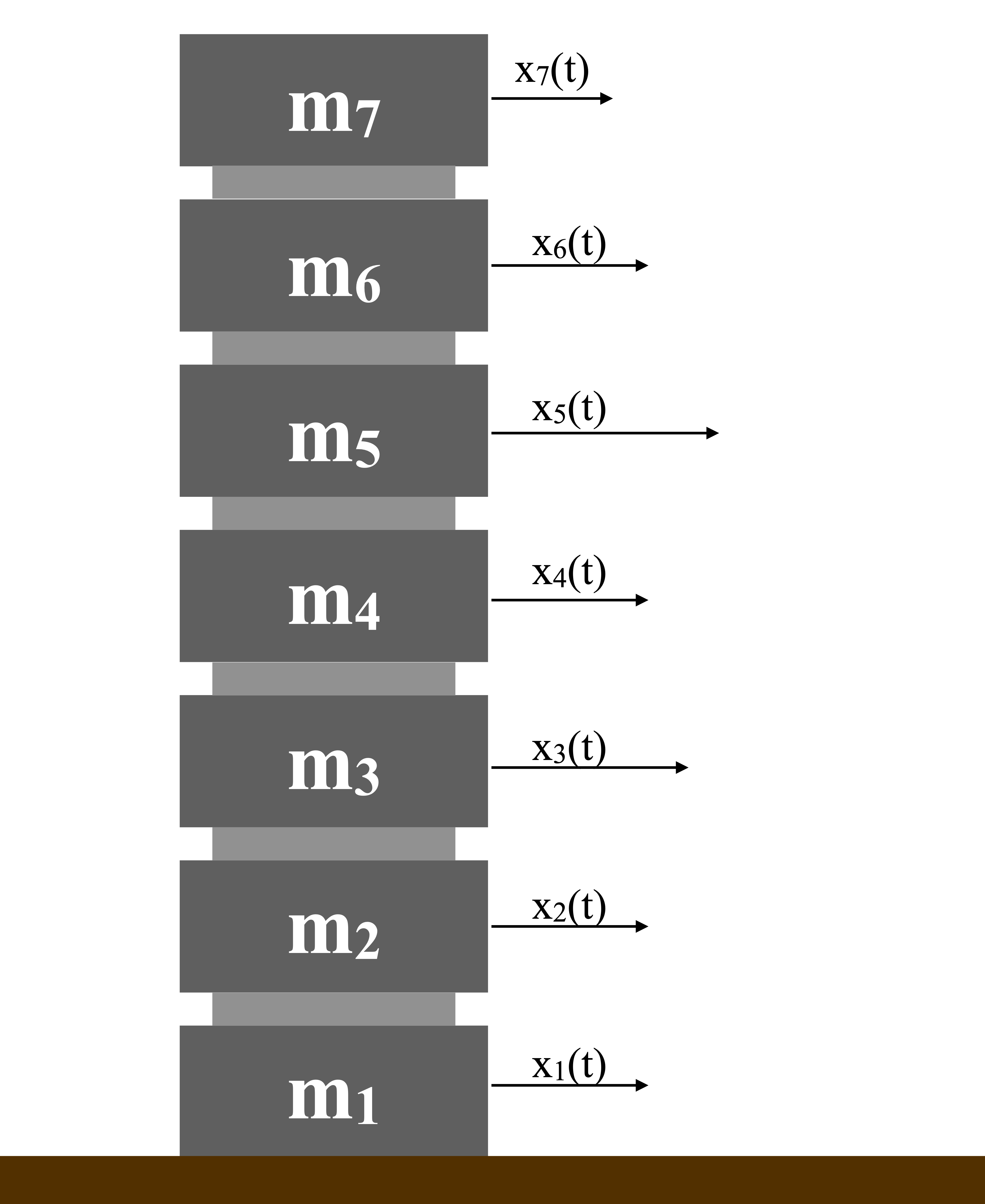
For example, with m=1000 and k=10000, we obtain the system
If this building is forced by an earthquake of frequency w, the acceleration on the ground floor (the first mass) will be proportional to w^2 \cos(w t):
where C_0 is the amplitude of the earthquake's acceleration on the building, and b is the vector
The particular solution will have the form x_p = \cos(w t) c where c is a vector of response amplitudes whose entries will depend on w; plugging in x_p we get
and we can equate coefficients of the cosine functions to get
The response is linear in C_0, so setting C_0 gives us the response per unit acceleration as a function of w. To sum up the overall response, we can use the length of the vector c. In terms of the period p = \frac{2 \pi}{w}, the response in our example looks like this:
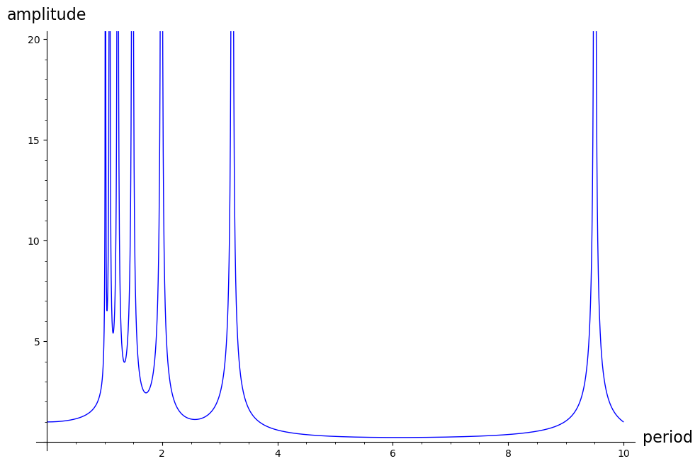
As this model has no damping, when w is equal to the frequency of a normal mode of the building the response amplitude is infinite.
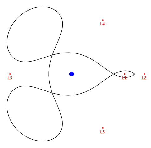
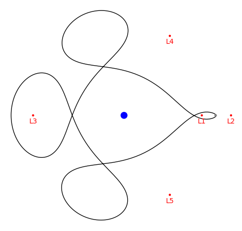
Numerical Example/Exercise: The restricted 3-body problem
The motion of two spherical masses interacting through Newtonian gravity can be more or less completely solved, with the famous result that they will move on conic curves (ellipses, parabolas, or hyperbolas). But for three bodies the motion is much more complicated; in some cases it is a fully chaotic system. However if one of the masses is zero (or in practical applications, very close to zero) quite a lot can be determined about the dynamics. This is called the restricted three-body problem.
The restricted 3-body problem model can be used as a relatively simple numerical model for predicting the motion of a spacecraft traveling near the Earth and Moon. The center of coordinates is the center of mass of the Earth-Moon system. A number of simplifying assumptions are made (corrections to which would slightly alter the actual behavior of a spacecraft):
- The influence of the Sun and other planets is ignored.
- The Earth and Moon have circular orbits.
- All motion takes place in a plane.
Special units of time and distance are chosen to make the equations simpler: the unit of time is one Earth-Moon revolution divided by 2 \pi, about 4.35 days. The unit of distance is the distance from the Earth to the Moon (about 384,000 kilometers). The units of mass are chosen so that the gravitational constant is 1. Finally, a uniformly rotating coordinating system is used so that the Earth is at the fixed location (-\mu,0) and the Moon is at (1-\mu,0) where \mu is the Moon's fraction of the Earth-Moon total mass, \mu = \frac{m_{M}}{m_E + m_M} \approx 0.0123. Using this rotating coordinate system introduces coriolus terms to the ODEs for the motion of the spacecraft as well as the gravitional accelerations:
Here r_E and r_M are the distances from the spacecraft to the Earth and Moon respectively.
The Matrix Exponential Viewpoint
A slightly different way of looking at systems of linear differential equations comes from looking at a basis of solutions as a matrix. If we start with a system of ODEs:
where A is a square n by n matrix and x is a vector, there is a n-dimensional space of solutions with a basis x_1(t), x_2(t), et cetera. Note that here the x_i are not components of x, but are each n-dimensional vector functions.
If we put all of these basis elements into a matrix X (i.e. the ith column of X is x_i), then that matrix satisfies the differential equation
Now recall that for the scalar first order ODE y' = a y, the solution is C e^{at}. We define a matrix exponential through the power series:
Similar to the scalar exponential, the factorial denominators increase quickly enough that this series converges for any matrix A. The solution to the matrix ODE is then
where C is any n by n constant matrix.
If we multiply a matrix solution X by a vector, we get a vector solution that is the linear combination of the columns of X. In particular, we can relate X to the other material in this chapter by noting that the initial value problem
where a_0 is a vector of initial values, has the solution
Suppose A is diagonalizable, so there is a matrix P of linearly independent eigenvectors v_i of A, and
where D is a diagonal matrix whose diagonal entries are the eigenvalues \lambda_i of A. Then
For the diagonal matrix D, e^{Dt} is easy to calculate - it is a diagonal matrix with diagonal entries e^{\lambda_i t}.
If we rewrite our initial conditions a_0 as the vector
then we recover the eigenvector-eigenvalue form
Additional Exercises
-
Find the general solution to the system x_1' = x_1 + 2x_2, x_2' = 2x_1 + x_2. Sketch some of the solutions near the origin, including some that start on the lines spanned by the eigenvectors of the coefficient matrix of the system.
-
Find the general solution to the system x_1' = x_1 + 2x_2, x_2' = 3x_1 + 2x_2.
-
Find the general solution to the system x_1' = x_1 - 5x_2, x_2' = x_1 - x_2. Sketch some of the solutions near the origin.
-
Solve the initial value problem x_1' = x_1 + 2x_2, x_2' = -2x_1 + x_2, x_1(0) = 1, x_2(0) = 0.
-
Suppose two 50 liter tanks are connected by two pumps which each transfer 10 liters/minute of fluid from each tank to the other. Suppose that the first tank initially contains 50 liters of brine at a concentration of 0.2 kg of salt per liter, and the other tank contains 50 liters of pure water.
a. Find the amount of salt in each tank as a function of time (you can assume that the tanks are well-stirred).
b. How long will it take for the amount of salt in the second tank to be within 1% of the amount of salt in the first tank?
-
Find the general solution of x' = Ax if
A = \left ( \begin{array}{cccc} 1 & 0 & 0 & 0 \\ 2 & 2 & 0 & 0 \\ 0 & 3 & 3 & 0 \\ 0 & 0 & 4 & 4 \end{array} \right ) -
Find the errors between the exact values of x_1(1) and x_2(1) and an approximation using Euler's method (with 2 steps) for the initial value problem
x_1' = 9x_1 + 5x_2,x_2' = -6x_1 - 2x_2,with x_1(0) = 0, x_2(0) = 1.
-
Suppose a rocket is fired (from height h=0) and after its initial burn it is at an altitude of h = 5 km with a velocity of 4 km/s straight up. Since it may reach a significant altitude, it could be too inaccurate to use a constant gravitational force. We will use the Newtonian law of gravity:
\frac{d^2h}{dt^2} = - \frac{g R^2}{(h+R)^2}where h is the height above sea level in kilometers, R = 6378 km, and g = 0.0098 km/s{}^2.
Convert this to a system of first-order equations and use a numerical method to find the maximum height of the rocket. Your answer should have two digits of accuracy (within the assumptions of the model). Use of computers (or a programmable calculator) is strongly encouraged for this problem.
9-10. For the last two problems, consider two blocks of mass m_1 and m_2 connected by springs to each other and to walls as shown below. The displacement of the masses from their equilibrium positions are denoted by x_1 and x_2. The stiffness of the three springs are k_1, k_2, and k_3 as shown. Compute the natural frequencies and describe the normal modes of oscillation in each of the three following cases:
-
k_1 = k_2 = 4 and k_3 = 2, and m_1 = 2, m_2 = 1.
-
k_1 = k_3 = 0 and k_2 = 4, and m_1 = m_2 = 1.
-
Consider a long cascade of tanks, each containing 1 liter of water. Each tank drains into the next at a rate of 1 liter per hour. Initially the first tank contains 1 gram of salt dissolved into it, but it is being refilled with pure water at a rate of 1 liter per hour. The other tanks in the cascade are initially filled with pure water. Compute how much salt is in the nth tank at time t.
Notes
Notes: (Local storage in a cookie)
License

This work (text, mathematical images, and javascript applets) is licensed under a Creative Commons Attribution-NonCommercial-ShareAlike 4.0 International License. Biographical images are from Wikipedia and have their own (similar) licenses.