First order ODE fundamentals

Mary Cartwright pic — Dame Mary Lucy Cartwright.

Introduction

Differential equations are mathematical relationships that involve changing quantities. To analyze these relationships we need tools from calculus - this is the main reason for calculus in the first place.

Historically differential equations arose from the study of physical phenomena such as: sound, the propagation of light, gravitation, electricity, magnetism, chemical reactions, and fluid dynamics. They are still heavily used for this purpose, but are also used for modeling financial processes (prices of stocks, bonds, and their derivatives), population dynamics and ecology, the spread of infectious diseases, pharmacology (pharmacokinetics), control (e.g. robotic motion), evolution, and many other applications.

There are two main types of differential equations, called ordinary and partial. An Ordinary Differential Equation, or ODE, only considers quantities which change relative to one independent variable. For example, near the surface of the Earth we can model the height $h$ of a freely falling object with the simple ODE model

$\frac{d^2 h}{dt^2} = - g$

where $t$ represents time and $g$ is the acceleration due to gravity (about $9.8$ meters per second per second). This model is a good example of a famous maxim "all models are wrong, but some are useful" (George Box). It entirely ignores air resistance, and we also know that the gravitational acceleration is not constant with respect to height, but it provides a useful and easy to solve model that is reasonably accurate for dense objects that are not moving very fast (for example, a cannonball dropped from rest by Galileo). We will return to this model later, and see the effect of improving it by adding in terms to represent air resistance.

Partial differential equations (PDEs) have more than one independent variable. A standard example is a model for the flow of heat ( $u$ ) in one dimension (perhaps modelling a metal bar or wire):

$\frac{\partial u}{\partial t} = k \frac{\partial^2 u}{\partial x^2}$

In this text we will focus on ODEs.

The simplest type of ODE is the kind you learn to do in calculus courses, which can be put in the form:

$\frac{d x}{d t} = f(t)$

These are solved by computing the integral of $f(t)$ . Even in this relatively easy and simple case we cannot always get a nice ("closed form") solution in terms of elementary functions - for example, the integral $\int \frac{1}{\ln(x)} dt$ cannot be written in terms of elementary functions (see the Wikipedia page for nonelementary integrals for more examples).

A practical word of advice for doing exercises and taking tests in this subject: avoid some of the most common mistakes in algebra and calculus.

1/f(x) integrals: e.g. $\int \frac{1}{sin{x}} dx$ IS NOT EQUAL TO $\log(\sin(x))$
exponential and log properties, e.g. $e^{a+b} = e^a e^b$ , and $\log(a^b) = b \log(a)$
algebra simplifications, e.g. $\frac{1}{a + b}$ IS NOT EQUAL TO $\frac{1}{a} + \frac{1}{b}$

Resources

Some other useful resources for learning about ODEs include:

MIT ODE lectures online

Essence of Linear Algebra 3Blue1Brown series

In the course I teach at UMD, we use Sage and Python in our computer lab exercises. A nice online introduction to Python is:

Interactive introduction to Python

Exercises

Calculate the second derivative of $f(t) = t^2 \cos(3t)$ .
Find the antiderivative of $te^t$ by integrating by parts.
Compute the integral $\int_0^1 \frac{2}{x^2 + x} \ dx$ by decomposing the integrand into partial fractions.

Separable ODEs

An ODE is called separable if its slope field factors:

$y' = f(x,y) = g(x) k(y)$

We can solve these ODEs, at least implicitly up to an integral. It is easier to work backwords from the solution. It also turns out to be more convenient to write the slope function as

$y' = g(x)/h(y)$

The implicit solution is

$\int h(y) dy = \int g(x) dx$

To see that this is equivalent to the differential equation, assume that we can write $y$ as a function of $x$ , and differentiate both sides with respect to $x$ . The right hand side simply becomes $g(x)$ , and for the left hand side we have to use the chain rule:

$\frac{d}{dx} \int h(y) dy = h(y) y' = h(y) g(x)/h(y) = g(x)$

There are two problems with solving separable ODEs: (1) it may be impossible to express the integrals in terms of elementary functions, and more importantly (2) it may be difficult or impossible to solve explicitly for the dependent variable.

Example: Exponential growth.

A population $P$ that can grow without constraint (i.e. it has plenty of every needed resource) will expand at a rate proportional to its population:

$\frac{d P}{d t} = k P$

Here the proportionality constant is $k$ . This is a separable equation, because the slope function does not depend on $t$ , so it is trivially factorizable (this is a special case called an autonomous ODE).

Before finding the solution $P = C e^{kt}$ using the separable technique, let us verify it is a solution. The derivative is $P' = k C e^{kt}$ , which is indeed $kP$ . It is often relatively easy to check that a solution is correct compared to finding it from scratch; this can be useful for example on an examination.

Separating the ODE gives:

$\frac{1}{P} \frac{d P}{d t} = k$

and then integrating both sides we get

$\ln(|P|) = k t + C_0$

This is an implicit solution; to get the explicit solution $P(t)$ we can exponentiate both sides. In this process of explicitly solving it is often useful to rename the arbitrary constant.

$|P| = e^{k t + C_0} = e^{C_0} e^{kt}$

and now if we drop the absolute value we may introduce a change of sign, which we can absorb into a new arbitrary constant $C_1 = \pm e^{C_0}$ ,

$$ P = C_1 e^{kt} $$

Example: Another Separable ODE.

Solve the initial value problem

$y' = \frac{x y^3}{\sqrt{1 + x^2}}, \ \ y(0) = -\frac{1}{2}$

To use the separability of this ODE we divide by $y^3$ and integrate:

$\int y^{-3} dy = \int \frac{x}{\sqrt{1 + x^2}} dx$

We can use the power rule for the left-hand side and the u-substituion $u = 1 + x^2$ for the right-hand side to get

$-\frac{1}{2 y^2} = \sqrt{1 + x^2} + C_0$

Before trying to solve for $y$ we can use the initial condition to determine $C_0$ :

$-2 = 1 + C_0$

so $C_0 = -3$ . Now we can solve for $y$ , although there are two possibilities for the sign when taking the square root:

$-\frac{1}{2 y^2} = \sqrt{1 + x^2} - 3$

$\frac{1}{y^2} = 6 - 2 \sqrt{1 + x^2}$

$y = \pm \frac{1}{\sqrt{6 - 2 \sqrt{1 + x^2}}}$

Since we want $y$ to be negative at $x=0$ , we need to choose the negative sign, so

$y = - \frac{1}{\sqrt{6 - 2 \sqrt{1 + x^2}}}$

Exercise

Which of the following ODEs are separable?

A. $y' = x + y$

B. $y' = x^2 + 2xy + y^2$

C. $y' = xy + 1$
Solve the separable differential equation $\frac{d y}{d x} = x y^2$ . Find the particular solution for which $y(0) = 2$ .

Slope Fields

A first order ODE:

$y' = f(x,y)$

expresses the requirement that the slope of the function $y$ must equal to $f(x,y)$ at each point $(x, y(x))$ of the solution. This can be visualized by drawing short arrows or line segments with slopes $f(x,y)$ at a grid of points. Much like a connect-the-dots picture, starting from an initial point we can connect the slopes to get an approximate solution.

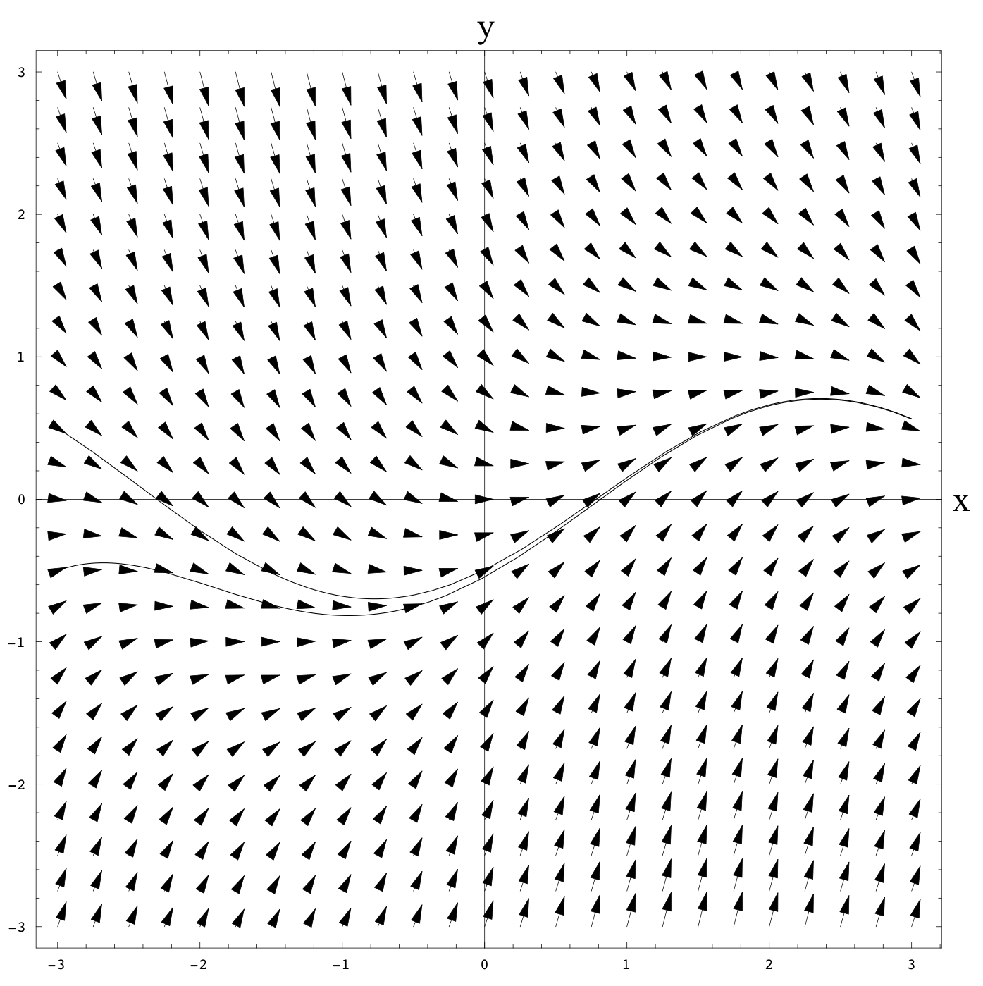
Shown below is the slope field for the ODE $y' = -y + \cos(x)$ .

Try a round or two of ODE golf.

Exercises: Slope field drawing and matching.

Sketch in the solution curves $y(x)$ with initial conditions $y(-3) = 1$ and $y(3) = 1$ . You can assume that separate solution curves never cross. Briefly describe how other solutions behave as $x$ increases.

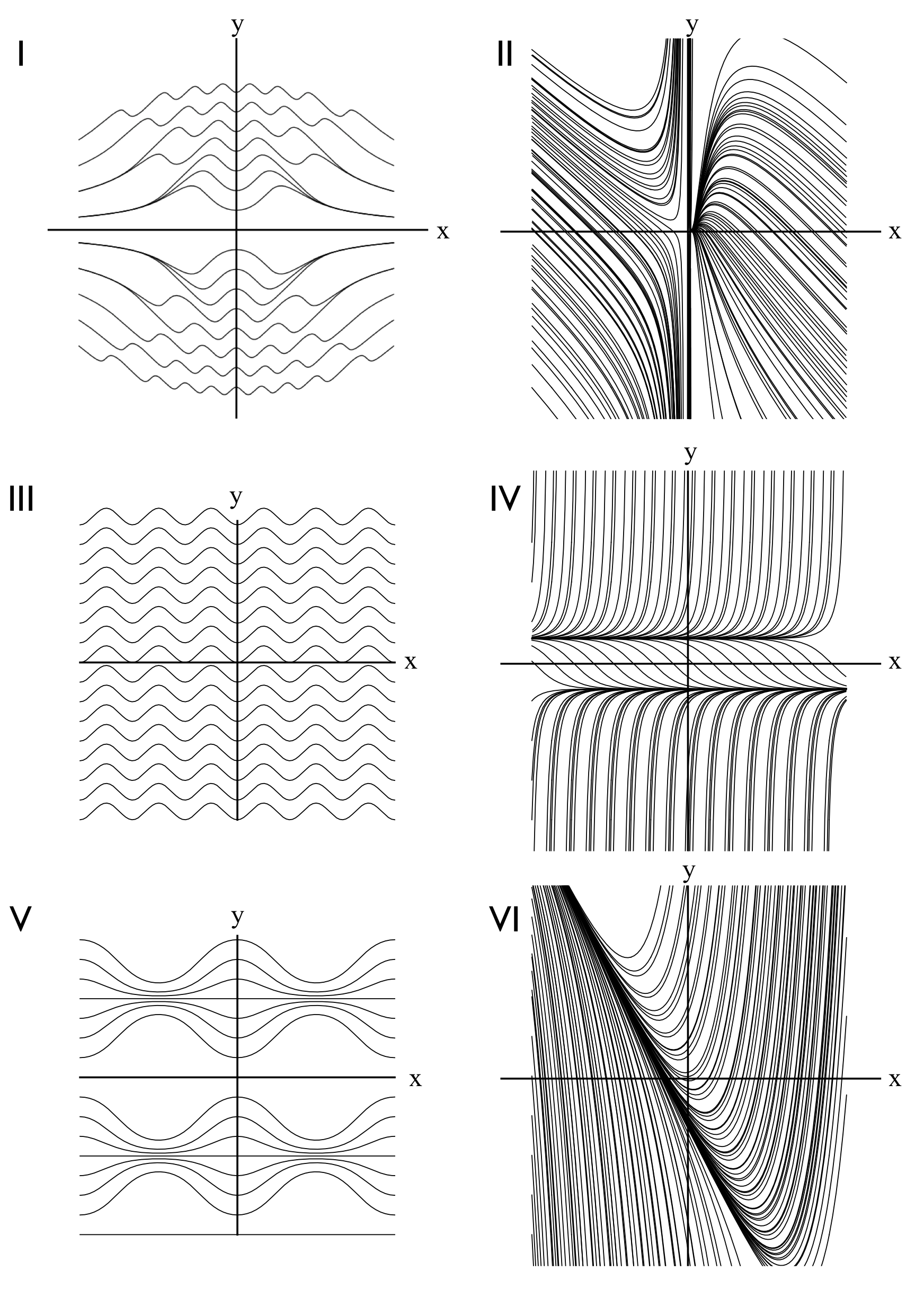
Match the following ODEs to the graphs below, which show some representative solutions. In each plot, the $x$ -axis is horizontal and the $y$ -axis is vertical. For each match briefly explain your reasoning. It may be helpful to consider things such as: what is slope equal to on each axis? Where is the slope 0?
1. $y' = \sin{(x y)}$
2. $y' = y^2 -1$
3. $y' = 2 x + y$
4. $y' = \sin{(x)}\sin{(y)}$
5. $y' = y/x^2-1$
6. $y' = \sin{(3 x)}$

Existence and Uniqueness

In this section we will be considering first-order ODEs, usually initial value problems in the particular form

$y' = f(t,y), \ \ \ y(t_0) = y_0$

We will refer to this simply as "the IVP".

It is helpful to know for any mathematical problem whether one can expect to find a solution, and if there could be more than one solution. This question is a bit more subtle for differential equations than a simple algebraic problem (such as a quadratic polynomial).

To illustrate one of the issues involved, let us consider the following example.

Example: The bucket problem.

Suppose that a bucket is filled with water to a height $y$ , and the bucket has a small hole at the bottom. If the bucket has a constant cross-sectional area then the height will satisfy the ODE:

$\frac{d y}{d t} = - k \sqrt{y}$

where $k$ is a positive constant that depends on the area of the hole and the units of $y$ and $t$ .

This is a separable ODE; to solve it we divide by $\sqrt{y}$ and integrate:

$\int \frac{1}{\sqrt{y}} dy = \int - k dt$

which yields the implicit solution˜

$2 \sqrt{y} = -kt + C_0$

Now we can solve for the explicit solution:

$y = (\frac{C_0 - kt}{2})^2$

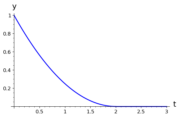
The solution seems mathematically pretty simple, but interpreting it raises some questions. If we start with the initial condition $y(0) = 1$ , then $C_0 = 2$ and we have

$y = (1 - kt/2)^2$

This solution has $y$ decrease until it becomes $0$ at $t=2/k$ , after which it seems the bucket starts (magically?) filling itself up. However this solution does not satisfy the ODE after $t=2/k$ . Intuitively of course we expect an empty bucket to stay empty, which corresponds to the constant solution $y = 0$ . It is simple to verify that $y=0$ is also a valid solution to the ODE. If we consider the initial condition to be $y(2) = 0$ , there are many solutions backwards in time, and only the zero solution forwards in time.

So overall the initial value problem with $y(0) = 1$ is quite tricky: we must switch at time $t=2/k$ to a different solution ( $y=0$ ) from that given by the separation method. A plot of this solution with $k=1$ is shown below.

Fortunately there are several precise theorems on when there are solutions to ODEs (existence theorems) and when there is exactly one solution (uniqueness theorems). We will summarize two of the simplest such theorems, the Peano existence theorem and the Picard uniqueness theorem.

Existence of solutions: The Peano existence theorem, proved by Giuseppe Peano around 1890, says that if the slope field $f(t,y)$ is continuous in an open set (e.g. an open disk in the $(t,y)$ plane) containing the initial condition $(t_0, y_0)$ , then there exists a solution $y(t)$ to the IVP in some interval of $t$ values containing $t_0$ .
Uniqueness of solutions: The Picard (or Picard-Lindelöf) theorem strengthens the Peano theorem: if the slope function $f(t,y)$ is both continuous and has a continuous partial derivative $\frac{\partial f}{\partial y}$ in an open set containing the initial condition, then there is a unique solution $y(t)$ to the IVP in some interval of $t$ values containing $t_0$ . This theorem was proved by Emile Picard around the same time as the Peano theorem (late 1800s).

Recall that the partial derivative of $f(x,y)$ with respect to $y$ is simply the derivative in the y-direction, with a fixed value of $x$ :

$\frac{\partial f}{\partial y} = \lim_{h \rightarrow 0} \frac{f(x,y+h) - f(x,y)}{h}$

Picard iteration (optional).

The Picard uniqueness proof uses a solution approximation technique called Picard iteration. We start with the constant approximate $y_0(t) = y(t_0)$ . Then for each function $y_i(t)$ , we get a better approximate solution $y_{i+1}(t)$ from:

$y_{i+1}(t) = y_i(t_0) + \int_{t_0}^{t} f(s, y_i(s)) ds$

(see below for an example of Picard iteration).

Example: Picard iteration

To see how Picard iteration works we will find some approximations to the solution of an IVP that we can explicitly solve:

$\frac{dy}{dt} = 2 y , \ \ y(0) = 1$

This is an example of exponential growth, with the solution $y = e^{2t}$ . The first three approximations from Picard iteration are:

First iteration:

$y_1 = 1 + \int_0^t 2 ds = 1 + 2t$

Second iteration:

$y_2 = 1 + \int_0^t 2(1+2s) ds = 1 + (2s + 2s^2)|_0^t = 1 + 2 t + 2 t^2$

And the third iteration gives:

$y_3 = 1 + \int_0^t 2(1 + 2s + 2s^2) ds = 1 + 2 t + 2 t^2 + \frac{4}{3} t^3$

This is the same as the first four terms of the power series of $e^{2t}$ at 0:

$e^{2t} = \sum_{n=0}^{\infty} \frac{2^n t^n}{n!} = 1 + 2 t + \frac{4 t^2}{2} + \frac{8 t^3}{6} \ldots$

One way to think about the uniqueness theorem is that solutions can't cross if they are unique. This can be helpful when thinking about the possible behavior of families of solutions with different initial conditions.

Example: Solution Intervals

Let us consider an example which shows that the interval on which a solution exists may be smaller than the region in which the slope field is continuous:

$y' = y^2, \ \ \ y(0) = 1$

In this example the slope function $f(t,y) = y^2$ only depends on $y$ , and it is infinitely differentiable at all points in the $(t,y)$ plane. So there is a unique solution to every initial value condition. We can find that solution by separation (dividing by $y^2$ ):

$\int y^{-2} dy = \int dt$

$- \frac{1}{y} = t + C_0$

We can plug in the initial condition here to find that $C_0 = -1$ , so

$y = \frac{-1}{t - 1} = \frac{1}{1 - t}$

This solution has a vertical asymptote at $t=1$ , so the solution to the IVP is only continuously defined for the interval $(-\infty, 1)$ .

Example: The bucket problem revisited

Let's reconsider the bucket problem from above in light of the Peano and Picard theorems. The ODE is

$y' = - k \sqrt{y}$

and we only consider $y$ in the domain $y \ge 0$ . Since the slope function is independent of $t$ , it is trivially continuous in that variable. For strictly positive $y$ , the function $\sqrt{y}$ is also continuous, so the Peano theorem guarantees that some solution exists for an interval of $t$ values around an initial condition with positive $y$ (and any value of $t$ ). The partial derivative of the slope function is $- \frac{k}{2\sqrt{y}}$ , which is also continuous for positive $y$ , so the Picard theorem says the solution will be unique.

However, if the initial value of $y$ is zero, then neither theorem applies and it is unclear whether a solution exists and whether any given solution is unique, since the functions $\sqrt{y}$ and $1/\sqrt{y}$ are not continuous in a neighborhood of zero (they aren't even defined for negative $y$ ).

Lets look a final example which has a rather spectacular failure of uniqueness for its solutions.

Example: A singular ODE

Suppose we wish to find solutions to the ODE

$t \frac{dy}{dt} = 2 y$

This is a separable ODE, and we can move the t and y to opposite sides from where they began and integrate:

$\frac{1}{y} \frac{dy}{dt} = 2 \frac{1}{t}$

$\log(|y|) = \int \frac{1}{y} dy = 2\int 2 \frac{1}{t} dt = \log(|t|) + C_0$

Now after exponentiating and using the fact that $e^{2 \log(|t|)} = t^2$ , we find that

$y = C_1 t^2$

where $C_1 = \pm e^{C_0}$ .

To we apply the Picard theorem to this problem, we need to write the ODE in the standard form $y' = f(t,y)$ , which in this case is:

$y' = \frac{2y}{t}$

The partial derivative of the slope function is

$\frac{\partial f}{\partial y} = \frac{2}{t}$

and we can see that both $f$ and $\frac{\partial f}{\partial y}$ are continuous functions except at $t = 0$ . So for any initial condition $y(t_0) = y_0$ there is a unique solution for some open interval of $t$ values containing $t_0$ ; we can solve for our constant $C_1$ to see that this solution is

$y = y_0(\frac{t}{t_0})^2$

However if $t_0 = 0$ , then either there are no solutions if $y_0 \neq 0$ , or infinitely many solutions if $y_0 = 0$ . This is a good example of the fact that if the conditions of Picard's theorem are not satisfied, it does not mean that the solutions are not unique - we cannot draw any particular conclusion in that situation.

Exercise: Existence and uniqueness for $y' = 3y^{2/3}t$ .

For the initial value problem $\frac{d y}{d t} = 3 y^{2/3} t$ , $y(1) = 1$ :

a. Find a solution to the IVP.

b. Determine the largest interval of $t$ values on which your solution from (a) is defined.

c. Does it have a unique solution? Check if the conditions of the Picard existence/uniqueness theorem apply. (Note this depends only on the slope function $f(t,y) = 3 y^{2/3} t$ , NOT the solution from part (a).)
Repeat the above problem, but this time with an initial value $y(1) = 0$ .

Linear First-Order ODEs

A linear first-order ODE with independent variable $x$ and dependent variable $y$ can be put into the standard form:

$\frac{d y}{d x} + P(x)y = Q(x)$

We can always solve this type of ODE, at least in terms of an explicit integration. One way to get this solution is to use a technique of Euler's called the integrating factor method. The idea of this method is to multiply the standard form by a function (the integrating factor $r(x)$ ) so that the left-hand side is a derivative of a product:

$\frac{d \ ?}{d x} = R(x) \frac{d y}{d x} + R(x) P(x)y = R(x) Q(x)$

What is the mystery product function in the left-hand side? It must be $r(x) y$ to match the first part of the derivative, which forces us into choosing $R'(x) = R(x) P(x)$ . This is a separable equation for $R$ , with the solution

$R(x) = C_R e^{\int P dx} = e^{\int P dx}$

and we can always choose $C_R=1$ since any nonzero choice of $C_R$ will give us the desired ability to rewrite the left-hand side as a derivative of a product. Then we can integrate both sides and divide by $R(x)$ to obtain

$\begin{equation}\label{lineq} y = \frac{C}{R(x)} + \frac{1}{R(x)} \int R(x) Q(x) dx \end{equation}$

Linear First-Order ODEs: a better perspective

An alternative, and more generalizable way to look at this formula, is to split the solution into two parts, $y = y_h + y_p$ , where $y_h$ solves the homogeneous ODE

$\frac{d y_h}{d x} + P(x)y_h = 0$

and $y_p$ is any one particular solution of the original ODE. The equation for $y_h$ is separable, with solution

$y_h = C_R e^{- \int P dx} = C_R/R$

To find the particular solution, we can use the "method of undetermined coefficients" by changing the constant coefficient $C_R$ of $y_h$ to an unknown function $u_p$ :

$y_p = u_p y_h$

Substituting this into the ODE we get

$\frac{d y_p}{d x} + P(x)y_p = \frac{d u_p}{d x} y_h + u_p \frac{d y_h}{d x} + P u_p y_h = Q(x)$

and using the fact that $y_h$ is the homogeneous solution this simplifies to

$\frac{d u_p}{d x} y_h = Q$

which can be integrated to find

$u_p = \int \frac{Q}{y_h} dx = C_R \int Q R dx$

We only need one choice of $u_p$ , and we can always choose the simple $C_R = 1$ . Since $y_p = u_p y_h$ , this means

$y_p = \frac{1}{R(x)} \int R(x) Q(x) dx$

and we have the same solution as before.

Example: Let us apply this formula to the ODE

$y' + \frac{x}{x^2+1}y = \frac{x}{x^2+1}$

with initial value $y(0) = 2$ . It is already in standard form (remember to make sure of this!), so we can see that $P(x) = Q(x) = \frac{x}{x^2+1}$ . Now we need to compute the integrating factor $R(x)$ (or equivalently $y_h = 1/R$ ):

$R = e^{\int P dx} = e^{\int \frac{x}{x^2+1} dx} = e^{\frac{1}{2} \log(x^2+1)}$

To integrate this we used the $u$ -substitution $u = x^2+1$ , so $\frac{d u}{d x} = 2 x$ . Since $a \log(b) = \log(b^a)$ , we can simplify $R$ :

$R = e^{\frac{1}{2} \log(x^2+1)} = e^{\log(\sqrt{x^2+1)}} = \sqrt{x^2+1}$

Now we need to be able to compute the integral $\int R Q dx$ . Often it is impossible to get an explicit solution to this integral, but in this example we can:

$\int R Q dx = \int \sqrt{x^2+1} \frac{x}{x^2+1} dx = \int \frac{x}{\sqrt{x^2+1}} dx = \sqrt{x^2+1}$

by using the same $u$ -substitution as before. Note that we can ignore the constant of integration here, since it is already included in the general formula for $y$ . So the general solution is

$y = \frac{C}{R(x)} + \frac{1}{R(x)} \int R(x) Q(x) dx = C (x^2+1)^{-1/2} + 1$

Finally we can plug in the initial condition to see that $y(0) = 2 = C + 1$ , so $C=1$ and $y = 1 + (x^2+1)^{-1/2}.$

Example: Newton's law of cooling: $T' = -k(T - A)$

An object hotter or cooler than its surroundings will exchange heat until it reaches the ambient temperature ( $A$ ). The simplest model for the rate of this heat exchange was posited by Isaac Newton in 1701, who assumed that it would be proportional to the temperature difference. This turns out to be a good model in many cases as along as the hotter object is not too hot - the radiative part of heat transfer increases proportionally to $T^4$ . An incandescent light bulb filament, for example, is around 3000 Kelvin when lit, and radiates about 10,000 times as much as it does at room temperature. For things below about 600 Kelvin (620 Fahrenheit), conduction is usually more important and Newton's heat 'law' works well.

The differential equation $\frac{d T}{d t} = -k(T - A)$ is both linear and separable. Using the linear formula, we first put it into the standard form: $\frac{d T}{d t} + k T = k A$ . The integrating factor is then

$R = e^{\int k dt} = e^{kt}$

and $$\int R Q dt = \int k e^{kt} A dt = A e^{kt} $$

Putting this into the linear solution formula, we get

$T = C e^{-kt} + A$

For an initial condition $T(t_0) = T_0$ , it is convenient to eliminate $C$ in terms of $t_0$ and $T_0$ and write the solution as:

$T = A + (T_0 - A) e^{-k(t - t_0)}$

Its a good exercise to derive this solution using the separation technique as well.

Exercise: linear ODE problem.

Compute $y(1)$ after solving the initial value problem $\displaystyle \ \frac{d y}{d x} = y + x$ , $y(0) = 1$ .

Substitution Methods and Exact ODEs

Throughout the 18th century, and well into the 19th century, many clever solutions to particular kinds of differential equations were found. In this section we will cover some of the most commonly arising and useful methods of these.

(This section will usually be skipped in Math 3280).

Homogeneous substitution

Perhaps the most useful method to be aware of is the method of homogeneous substitution. If a differential equation can be written in terms of the quantity $v = \frac{y}{x}$ , then the derivative

$\frac{d v}{dx} = \frac{1}{x} \frac{d y}{d x} - \frac{y}{x^2} = \frac{1}{x} \frac{d y}{d x} - \frac{v}{x}$

or equivalently

$\frac{d y}{d x} = v + x \frac{d v}{d x}$

After replacing $y$ and $\frac{d y}{d x}$ with $v x$ and $v + x \frac{d v}{d x}$ respectively, we obtain a separable equation.

Example: Homogeneous substitution

We will solve the initial value problem

$x y \frac{dy}{dx} = 2 x^2 + \frac{3}{2} y^2$

$y(1) = 1$

using the homogeneous substitution method. First we can divide the ODE by $x y$ , and replace $y$ with $v x$ to get

$\frac{dy}{dx} = 2 \frac{x}{y} + \frac{3}{2} \frac{y}{x} = \frac{2}{v} + \frac{3}{2}v$

Now replacing $\frac{d y}{d x}$ by $v + x \frac{d v}{d x}$ , we get

$v + x \frac{d v}{d x} = \frac{2}{v} + \frac{3}{2}v$

Now we can rearrange this into the separated form

$\frac{2v}{v^2 + 4} \frac{d v}{d x} = \frac{1}{x}$

and integrate both sides to get

$\log(v^2 + 4) = \log|x| + C_0 .$

We now want to solve for $v$ . To start, we can use both sides to exponentiate $e$ , cancelling the logarithms, and get

$v^2 + 4 = C_1 |x|.$

To get the answer in terms of the original variable $y$ , we can replace $v$ by $y/x$ and relax the sign constraint left over from exponentiating to get:

$y^2 + 4 x^2 = C_2 x^3 .$

Plugging in our initial condition shows that we need $1 + 4 = 5 = C_2$ , so the solution with positive $y$ values is

$y = \sqrt{5 x^3 - 4 x^2} .$

Bernoulli equations

If an ODE can be put into the form

$\frac{dy}{dx} + P(x) y = Q(x) y^n$

then it can be converted into the linear ODE

$\frac{dv}{dx} + (1-n) P(x) v = (1-n) Q(x)$

by the substitution $v = y^{n-1}$ . This is usually called a Bernoulli differential equation, even though Leibniz was the first to notice this solution technique (one of many examples of somewhat mis-named results in mathematics).

Bernoulli equation example

We will illustrate the Bernoulli substitution on the ODE

$y' = y + e^{-2t}y^2$

This particular example is also a Ricatti equation, which are ODEs with at most constant, linear, and quadratic terms.

Here the exponent $n=2$ , so we use $v = y^{-1}$ . The ODE in terms of $v$ is then

$v' = - v - e^{-2t}$

This nonhomogeneous linear equation can be solved with the integrating factor method. In the standard $v' + Pv = Q$ form we have $P=1$ and $Q=-e^{-2t}$ . The integrating factor is $R = e^{\int P dt} = e^t$ , and

$v = \frac{C}{R} + \frac{1}{R} \int R Q dt = C e^{-t} + e^{-2t}$

Transforming back to $y = v^{-1}$ gives us

$y = \frac{1}{C e^{-t} + e^{-2t}}$

Note that if $y(t_i) = 0$ , then we cannot solve for a value of $C$ that satisfies the initial condition; this is not too surprising since our substitution technique was not well-defined for $y=0$ . But in this case we can check that the constant $y=0$ is a solution.

Exact ODEs

An implicitly defined curve

$F(x, y(x)) = 0$

gives rise (via implicit differentiation with respect to $x$ ) to the ODE:

$\frac{\partial F}{\partial x} + \frac{\partial F}{\partial y} \frac{dy}{dx} = 0 .$

If we are considering a differential equation

$M(x,y) + N(x,y) \frac{dy}{dx}$

then we can view it as coming from an implicit curve if the partial derivatives are compatible with the fact that $\frac{\partial^2 F}{\partial x \partial y} = \frac{\partial^2 F}{\partial y \partial y}$ (Clairaut's theorem), i.e. if

$\frac{\partial M}{ \partial y} = \frac{\partial N}{ \partial x} .$

If the above conditions hold, the differential equation is called closed, and on a simple domain in the x-y plane such as a rectangle, it is also exact, meaning the solution can be desribed by an implicit curve $F$ .

Example of an exact ODE

The differential equation

$3 x y^2 \frac{d y}{d x} = - y^3$

is exact, with $M = y^3$ and $N = 3 x y^2$ . We can check that

$\frac{\partial M}{ \partial y} = \frac{\partial N}{ \partial x} = 3 y^2$

The implicit function $F$ must satisfy

$\frac{\partial F}{\partial x} = y^3$

and

$\frac{\partial F}{\partial y} = 3 x y^2,$

which is only possible for $F = x y^3 + C_0$ . In this case, we can solve the implicit equation $F=0$ for $y$ to get

$y = - (C_0/x)^{1/3} = C_1 x^{-1/3}.$

Additional Exercises

Verify that $y = 2e^{-3x}$ is a solution to the ODE $y' = -3y$ .
Find all solutions of the form $y = e^{rx}$ to the differential equation $3y'' - 4y' -4y=0$ by substitution. ( $r$ is a constant you need to determine the possible values of.)
Find all solutions of the form $y = e^{rx}$ to the differential equation $3y'' - 4y' -4y=0$ by substitution. ( $r$ is a constant you need to determine the possible values of.)
Determine a value of the constant $C$ so that the given solution of the differential equation satisfies the initial condition.

a. $y = \ln(x + C)$ solves $e^y y' = 1$ , $y(0) = 1$ .

b. $y = Ce^{-x} + x - 1$ solves $y' = x - y$ , $y(0) = 3$ .
Write a differential equation for a population $P$ that is changing in time ( $t$ ) such that the rate of change is proportional to the square root of $P$ .
Solve the initial value problem $\frac{d y}{d x} = 3x + 1$ , $y(0) = 1$ .
Solve the initial value problem $\frac{d y}{d x} = \sqrt{x}$ , $y(9) = 0$ .
Solve the initial value problem $\frac{d y}{d x} = \frac{1}{\sqrt{1-x^2}}$ , $y(0) = 0$ .
Solve the initial value problem $\frac{d y}{d x} = x e^{-x}$ , $y(0) = 2$ .
Find the general solutions $y(x)$ to the separable ODE $y' = 4xy$ .
Find the general solutions $y(x)$ to the separable ODE $(2+2x)y' = 4y$ .
Find the general solutions $y(x)$ to the separable ODE $y' = y \cos(x)$ .
Find the general solutions $y(x)$ to the separable ODE $y' = 1 + x + y + xy$ .
Find the solution $y(x)$ to the initial value problem $y' = 2 y e^x$ , $\ y(0) = 2e^2$ .
Find the solution $y(x)$ to the initial value problem $y' = x^3 (y^2+1)$ , $\ y(0) = 1$ .
In carbon-dating organic material it is assumed that the amount of carbon-14 ( ${}^{14}C$ ) decays exponentially ( $\frac{d \ {}^{14}C}{dt} = - k\ {}^{14}C$ ) with rate constant of $k \approx 0.0001216$ where $t$ is measured in years. Suppose an archeological bone sample contains 1/7 as much carbon-14 as is in a present-day sample. How old is the bone?
Suppose you are designing a dosage regimen for the antibiotic ciprofloxacin (cipro). Assume the half-life of cipro is 4 hours. Let $x(t)$ be the amount of cipro present at time $t$ hours after the initial dose, in units of milligrams per kilogram of the patient, and that $x$ satisfies the differential equation $x' = -kx$ where $k$ is a constant. If you decide to use equal doses which increase the value of $x$ by $10$ every $4$ hours, how large can $x$ become over time?

18 - 21: Determine what the existence and uniqueness theorems guarantee about solutions to the following initial value problems (note that you do not have to find the solutions:
(see above) $dy/dx = \sqrt{xy}$ , $y(0) = 1$ .
(see above) $dy/dx = y^{1/3}$ , $y(0) = 2$ .
(see above) $dy/dx = y^{1/3}$ , $y(2) = 0$ .
(see above) $dy/dx = x \ln(y)$ , $y(0) = 1$ .
Solve the first-order linear ODE $dy/dx = -2 y + 2xe^{-2x}$ .
Solve the first-order linear ODE $dy/dx + y \tan(x) = \sin(x)$ .
Solve the linear initial value problem $xy' = y + 2x$ , $\ y(1) = 2$ .
Solve the linear initial value problem $y' + 4 y = 2xe^{-4 x}$ , $\ y(0) = 0$ .
Solve the linear initial value problem $y' = \cos(x) - y \cos(x)$ , $\ y(0) = 1$ .
Solve the linear initial value problem $y' = 1 + 2xy$ , $\ y(0) = 1$ . Your answer can be written in terms of the error function, $\text{erf}(x) = \frac{2}{\sqrt{\pi}} \int_0^{x}e^{-t^2}dt$ .
Consider a tank containing $1000$ liters (L) of brine with $100$ kilograms (kg) of salt dissolved. Pure water is added to the tank at a rate of $10$ L/s, and stirred mixture is drained out at a rate of $10$ L/s. Find the time at which only $1$ kg of salt is left in the tank.
Consider two tanks, with the first tank draining into the second. The first tank has $10$ liters of a solution containing $200$ grams of a dye dissolved in it. It drains into the second tank at a rate of $1$ L/s, while being refilled with pure water at the same rate. The second tank initially contains $100$ liters of pure water and is being emptied at a rate of $1$ L/s. Both tanks are well-stirred at all times. Find the maximum concentration of dye in the second tank.
Use (a) Euler's method and (b) the 4th-order Runge-Kutta method to estimate $x(1)$ if $\ x(0) = 1$ and $\frac{d x}{d t} = x + t^2$ , using $2$ steps. For this question you can use a calculator but you should write out the steps explicitly.
Suppose a population of invasive gophers, P, grows at a rate proportional to the square root of the population. Initially the population size is 400 and it is increasing (initially) at a rate of 40 gophers/month. What will the population be after 1 year?

(This dependence is sometimes used for a geographically expanding population, in which there is an internal population plateaued at its maximum sustainable level surrounded by a thin zone of colonization. The size of the thin zone is proportional to the square root of the internal area.)
Suppose a population of 15000 people are susceptible to a contagious disease, and that this disease spreads at a rate that is proportional to the number of infected people times the number of uninfected people. If there are initially 1000 people with the disease, and the number of infections is increasing at a rate of 140/day, how much longer will it take for half the population to be infected?

Notes

Notes: (Local storage in a cookie)

License

This work (text, mathematical images, and javascript applets) is licensed under a Creative Commons Attribution-NonCommercial-ShareAlike 4.0 International License. Biographical images are from Wikipedia and have their own (similar) licenses.