Applications and numerical approximations

Compartment models

In this section we use linear ODEs to model interacting compartments ("tanks") of various types. Our examples will mostly consist of tanks full of liquid solutions, such as salty water, but mathematically similar models are used to model population dynamics, disease transmission, pollution, economic sector activities, and many other things.

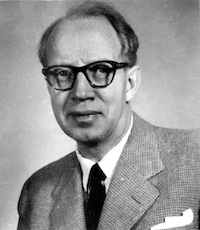
The use of compartment models in pharmacokinetics (how concentrations of drugs change in an organism over time) was pioneered by the Swedish physiologist Torsten Teorell in the late 1930s.

---

Example: Tank problem

Consider a 120 L tank initially filled with 90 L of brine at a concentration of 1 gram/liter. There is an inflow of brine at 2 grams/liter at a rate of 4 liters/minute, and an outflow of well-mixed brine at 3 liters/minute. Find the amount of salt in the tank when the tank is full.

In any compartment/tank problem, it helps to break down the inputs and outputs separately. In this case we have one inflow, and one outflow. The quantity we want to track is the amount of salt in grams in the tank; lets call that $x$. The amount of salt coming in is the (inflow rate)*concentration, which is $2$ times $8$. So

The amount leaving the tank is the (outflow rate)*concentration. The outflow rate is $3$ liters/minute. The concentration is the amount of salt in the tank divided by the volume of fluid in the tank. How much salt is in the tank? That is what we are trying to find out, its $x$. The volume, $V$, of fluid in the tank is increasing because there is more fluid coming in to the tank than there is going out. In fact we could write a little mini-IVP for the volume:

which we can integrate to get $V = 90 + t$. So our ODE for the salt is

with initial condition $x(0) = 90$ since initially there is 90 liters of fluid with a concentration of 1 gram/liter.

Now we can put the ODE in standard linear form $x' + P(t)x = Q(t)$:

The integrating factor is

Make sure you understand that last step! It is a very common error to simplify this incorrectly.

The other integral we need to compute is $\int Q(t) R(t) dt$, which we can do with a $u$-substitution:

The solution is

The penultimate step is finding the value of the constant $C_0$. We know that $x(0) = 90$, which means that

so

So the amount of salt is

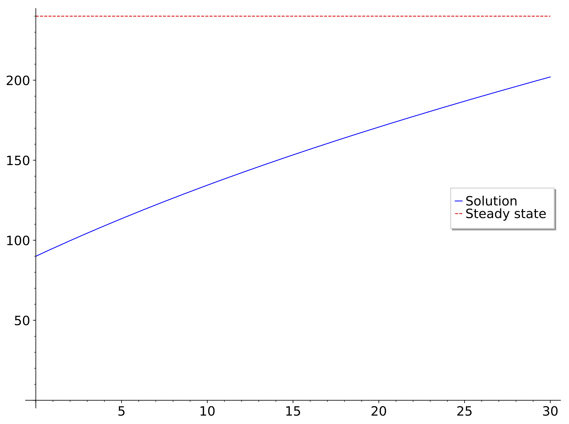
and our final answer is the amount of salt when the tank is full, which happens at $t=30$ minutes:

If we let the tank overflow, or began draining it more at $t=30$ to keep the volume at 120 L, it would approach a steady-state concentration of $2$ g/L salt - the total salt in the tank would be 240 g. Below is the plot of the solution with this steady-state amount drawn as a dashed red line.

---

Exercise:

One tank draining into another.

1. Consider a pair of tanks in which tank 1 drains into tank 2 at a rate of 5 liters/minute. Tank 1 intially contains 100% ethanol, but is being refilled with pure water at a rate of 5 liters/minute. Tank 2 initially has pure water in it and drains at a rate of 5 liters/minute. Tank 1 has a volume of 100 liters, and tank 2 has a volume of 10 liters.

   A. Write down ODEs for the amount of ethanol in each tank and solve them. (Note that the amount in tank 1 does not depend on the amount in tank 2.)

   B. Find the maximum amount of ethanol present in tank 2 (first find when this happens).

Euler's Method

Most differential equations, and systems of differential equations, do not have an explicit solution. It is therefore essential to have some understanding of methods to approximate solutions numerically. The simplest such method is known as Euler's Method. As we will see, it is not a good method, but it is important to have a solid understand of it before considering more complicated alternatives.

The standard form for a first-order initial value problem (IVP) is:

Euler's Method relies on a tangent-line approximation to the solution at each approximation point $(x_i, y_i)$ to obtain the next point $(x_{i+1}, y_{i+1})$:

where $h$ is the stepsize in the $x$ variable. In this text we will usually choose a fixed stepsize $h$, although in more advanced methods it is useful to change $h$ adaptively.

---

Example: Euler's method

For the IVP $$ y' = y + x, \ \ \ y(0) = 1 $$

use Euler's method to find $y(2)$ in $1$, $2$, and $4$ steps.

• 1 step: For this, $h = \frac{2 - 0}{1} = 2$.

• 2 steps: Now $h = 1$. For the first step,

Then for the second step:

Finally if we take four steps, $h = 1/2$:

Step 1:

Step 2:

Step 3:

Step 4:

The exact solution to this problem is $y = 2e^x - x -1$, so

So we can see that the 4-step Euler's Method is not doing a very good job. Fortunately, there are a plethora of methods that are generally much better.

---

In the frame below we show the exact solution to the initial value problem

which is $y = \cos(3x)$, and some approximations using Euler's Method.

Exercises:

1. Use Euler's method to estimate $y(1)$ if $\ y(0) = 1$ and $\frac{d y}{d x} = \frac{y}{2-x} + x^2$, using $1$, $2$, and $4$ steps.

2. Find the exact value of $y(1)$ by solving the initial value problem (note that the ODE is linear).

Improved Euler's Method and the Runge-Kutta 4th Order Method

At every step Euler's method will be in error by an amount that is usually dominated by the magnitude of the derivative of its slope function along the solution - the second derivative of the solution $y(x)$. At each step the error bound is proportional to $h^2$; over a fixed solution interval $[x_0, x_f]$ after taking $n$ steps of stepsize $h$ the total error bound is:

for some constant $M$ that depends on $f(x,y)$. So we expect the error to decrease linearly with $h$, once $h$ becomes small. In general, if a method has an error bound of the form:

then we say it has order $p$.

There are many different methods of higher order than Euler's Method; we will only discuss two of the simpler ones, the somewhat sadly named "Improved Euler's Method" and the fourth-order Runge-Kutta method.

• The Improved Euler's Method uses at each step two estimates of the solution slope between the points $(x_i, y_i)$ and $(x_{i+1}, y_{i+1})$:

and simply averages them to obtain the next point:

Example: Improved Euler's method

Let's look at the same example as before, the initial value problem

$$ y' = y + x, \ \ \ y(0) = 1 $$ but this time use the Improved Euler's method with two steps to approximate $y(2)$.

Going from $x=0$ to $x=2$ in two steps means that our stepsize $h=1$.

For the first step, $x_0 = 0$ and $y_0 = 1$ and the slopes are

So $x_1 = x_0 + h = 0 + 1 = 1$ and

For the second step, the slopes are

and we have $y(2) \approx y_2 = 3 + \frac{4 + 9}{2} = 9.5$

Since the exact solution is about $11.778$, we can see that just two steps of this method get much closer to the correct answer than four steps of Euler's Method.

---

The 4th-order Runge-Kutta method

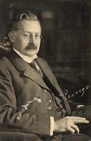
The final method we will look at is the 4th-order Runge-Kutta method, developed by Carl Runge and Martin Kutta in the early 1900s. This method is part of family of methods; we choose the 4th order method because it has a good balance of simplicity and accuracy (any higher order method becomes very tedious to do by hand).

$\frac{dy}{dx} = f(x,y)$, going from $(x_i, y_i)$ to $(x_{i+1}, y_{i+1})$ with stepsize $h$ are:

And then:

---

Runge-Kutta 4th order method example

Once again we will use the initial value problem

and approximate $y(2)$ using two steps of the Runge-Kutta 4th order method.

At each step we need to compute four slopes. As before, we start with $x_0=0$, $y_0=1$, and $h=1$. For step one, the four slopes ($k_i$) are:

Now we use the weighted average of these to find $y_1$:

For the next step we only need the values $x_1 = 1$ and $y_1 = 41/12$. We will keep these computations exact to show the steps more clearly, but in practice all of these numerical methods are usually done with floating-point numbers.

Finally, we can compute $y_2$:

Since $\frac{3361}{288}$ is approximately $11.67$, we can see that this method gets much closer than the previous ones to the exact answer $y(2) \approx 11.778$.

---

Exercise: Improved Euler method and RK4.

1. For the initial value problem $y(1) = 1$ and $\displaystyle \frac{d y}{d x} = \left ( \frac{y}{x}\right ) \left ( \frac{y - x}{x + y} \right )$, approximate $y(2)$ by using:

   1. 1 step of the improved Euler method

   2. 1 step of the 4th-order Runge-Kutta method (formulae on reverse).

Equilibria and Stability

An autonomous first ODE can written in the form

i.e. the slope function only depends on the dependent variable $y$. This is very common in modeling, where time ($t$) does not directly affect the state of a system. These ODEs are always separable, but apart from very simple cases it is usually impossible to explicitly invert the implicit solution

Even when it is possible to solve for $y$, it may not be much more useful than the qualitative understanding we obtain from an analysis of the equilibria, where $f(y) = 0$, and their stability. Let us start by analyzing a famous and useful example.

---

The logistic equation.

The logistic model is commonly used for populations growing in a stable environment. In this model there is assumed to be a finite amount of resources (space, food, et cetera), and consequently the population has a "carrying capacity" of $M$. If the population ($P$) is larger than $M$, it will decrease. For small values of $P$, the population grows exponentially. The logistic model is the simplest one with those characteristics:

We can explicitly solve this, by separation, although quite a few steps are required: the integral is done by partial fraction decomposition, and then some properties of logarithms and exponentials are needed to simplify the answer:

and now we divide by $e^{Mkt}$ and use the initial condition $P(0) = P_0$ to replace $C_2$:

---

Stability

One of the most important properties of an equilibrium point is its stability: do nearby solutions stay near the equilibrium, or move away? There are many technical definitions of stability, especially in more than one dimension. We will use a definition of local stability in one dimension that is easy to check: an equilibrium point $y_e$ for the system $y' = f(y)$ (i.e. $f(y_e) = 0$) is stable if there is an $\epsilon$ such that $f(y) \ge 0$ for $y \in (y_e - \epsilon, y_e)$, and $f(y) \le 0$ for $y \in (y_e, y_e + \epsilon)$.

In between the equilibria, if the slope function $f(y)$ is continuous it will be either positive or negative in each interval. Then we only need to check the sign for one point in each interval.

---

Example: Equilibria and stability

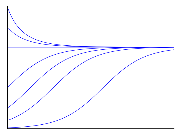
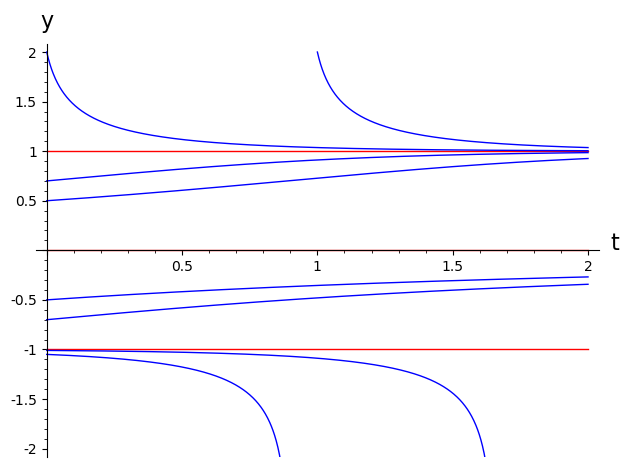
Here is another example of an autonomous system (not from any particular application):

Finding the explicit solution to this takes quite a bit of effort (partial fraction decomposition, integration to an implicit solution, and then difficult algebra to solve for $y$ explicitly. In contrast, analyzing the equilibria and their stability is relatively easy.

The equilibria are the roots of $f(y) = y^2 - y^4 = 0$, which can be factored as $y^2(1-y^2) = y^2(1+y)(1-y) = 0$ with roots $-1$, $0$, and $1$.

We can determine whether a solution is increasing or decreasing between these equilibria by checking the slope function's sign anywhere between them. For example, since $f(-2) = 4 - 16 = -12 < 0$, solutions that begin below $y=-1$ will always decrease. Since $f(-1/2) = f(1/2) = 1/4 - 1/16 > 0$, solutions increase both below $y=0$ and above $y=0$. Finally, since $f(2) = -12 < 0$ solutions above $y=1$ decrease. We can summarize all of this in a "phase diagram" showing the equilibria and solution directions

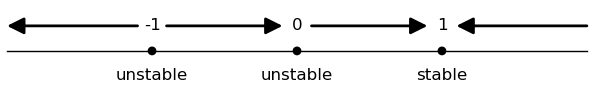
The phase diagram has $y$ as its horizontal axis, which can be a little confusing. Usually we plot solutions $y(t)$ with $t$ horizontal. If we rotate the phase diagram, the slope information enables us to sketch solutions. For this example, this is shown below, with the equilibria solutions in red.

---

Exercises: Equilibria and phase plots

1. Sketch the phase plot (equilibria and direction of solutions) for the ODE $y' = y \sin{y}$ in the interval $y \in [-10,10]$.

2. Sketch the phase plot (equilibria and direction of solutions) for the ODE $y' = y^9 - y$ in the interval $y \in [-2, 2]$.

---

Bifurcations of Equilibria

A bifurcation in a family of parameterized differential equations is where the number or type (stability) of equilibria change. In general many sorts of bifurcations are possible, but there are a few common types of bifurcations that occur generically. In higher dimensions the study of bifurcations is a significant area of research mathematics. In one dimension there are not too many possibilities. In the example below we will see one of the very common 1-D bifurcations, the saddle-node bifurcation, in which a stable and unstable pair of equilibria coalesce and annihilate.

---

Example: The logistic harvesting problem

Suppose a population $P$ is modeled by the logistic equation with a carrying capacity $M$, and we choose units of time so that $k=1$. We can also choose the unit of population so that $M=1$. What happens if this population (of fish, for example) is harvested at a certain rate $h$? We can examine the location and stability of the equilibria as a function of $h$ without needing to explicitly solve the ODEs.

First we find the equilibria:

and from the quadratic formula we find that the equilibria $P_{\ast}$ are

$$P_{\ast} = \frac{1}{2} \left ( 1 \pm \sqrt{1 - 4h} \right ) $$

For $h < 1/4$, there are two equilibria. At these two equilibria we can calculate the derivative of the slope field with respect to population:

and the sign of these derivatives means that the larger equilibrium is stable and the lower unstable. When the number or stability of the equilibria changes it is called a bifurcation. In this case we have a bifurcation at $h=1/4$. If we plot this family of systems in the $h,P$ plane, we have a bifurcation diagram. An animated version for this system is shown below.

---

Exercise: $-hP$ harvesting term

1. Suppose that before fishing is allowed, a population of fish in a lake satisfies the differential equation $\displaystyle \frac{d P}{d t} = P(1000-P)$ where $t$ is measured in years. Then fishing is allowed at a rate proportional to the population, so that $\displaystyle \frac{d P}{d t}$ is decreased by $hP$ where $h$ is a parameter.

   a. Sketch a bifurcation diagram in the $(h,P)$ plane that shows the equilibria of the system as $h$ is varied and their stability.

   b. If $h = 500$, and the lake begins in an overstocked state with $P = 2000$, what value will the population approach over time?

   c. If $h = 1000$, and the lake begins in an overstocked state with $P = 2000$, what value will the population approach over time?

Air resistance models

We will consider three models for air resistance, for some object in motion near the Earth's surface. The only other force included in our model will be that of gravity.

As a baseline let's review the kinematics of a body under the force of gravity without any air resistance. The gravitational force on a body of mass $m$ towards the Earth (mass $m_E$) in the vertical direction is

where $R_E$ is the radius of the earth, $G$ is the universal gravitational constant, and $y$ is the height of the object above the Earth's surface. Unless the object is a spacecraft the height $y$ is usually very small compared to the Earth's radius, and we approximate the acceleration of the object by a constant $g$:

In SI units $g$ is $9.8$ meters per second per second.

If we use the constant surface acceleration approximation it is relatively simple to get equations for the velocity $v = h'$ and height $h$ as functions of time by direct integration:

Linear air resistance

For most purposes it is unacceptably inaccurate to ignore air resistance entirely. The simplest useful model for air resistance is a frictional acceleration in the opposite direction to the motion that is linearly proportional to the velocity:

We have chosen to name the proportionality constant $r$. This ODE is both separable and linear (with constant coefficients), so we have a number of ways to find the solution. Using the integrating factor method for linear ODEs, we first put it into the standard linear form:

The integrating factor is $R = e^{\int r dt} = e^{rt}$, and the general solution is

where the second form has been rewritten in terms of the initial velocity $v(0) = v_0$. We can see that as the time $t$ increases, the exponential $e^{-rt}$ will become small, and the velocity will approach the constant $-g/r$, which is often called the terminal velocity.

Now to find the height we need to integrate $v(t)$, which gives us

where again instead of the arbitrary constant $C_1$ we have written $h$ in a second form which is more convenient if we have an initial height $h(0) = h_0$.

Quadratic air resistance

For objects moving very quickly through a thin medium (such as the upper atmosphere) the air resistance is better approximated as a quadratic function of the velocity:

where $k$ is a positive constant and the sign function $sgn$ is defined to be $1$ for a positive input, $-1$ for a negative input and $0$ if the input is zero. Equivalently we could use $v |v| = v^2 sgn(v)$. This ODE is nonlinear but still separable, so we can write an implicit solution:

The details of the integral now depend a little on the sign of $v$. In our opinion however this is not worth spending too much time thinking about, because this model is not very realistic anyway. If it is worth your time to get an accurate model for air resistance you are better off using the next subsection's model.

General air resistance

If it is important to model air resistance very accurately, we can do better than the linear or quadratic models. In general the fluid mechanics that are responsible for air resistance are extremely complex, and do not reduce to a simple power dependence on velocity. A full fluid mechanical simulation is far beyond the scope of this text. We will instead briefly present a useful practical approximation that does a good job modeling many objects over a wide range of velocities.

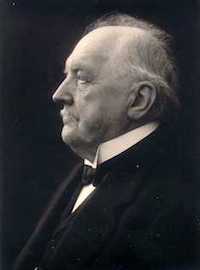
The approximation is posed in terms of an important fluid mechanics quantity called the Reynolds number, named after the UK professor (one of the very first professors of engineering) Osborne Reynolds. The Reynolds number is a dimensionless number that is proportional to velocity:

where $l$ is length of object (usually use the diameter), $\mu$ is viscosity of the fuild medium, $\rho$ is the fluid density, and $v$ is the speed of the object through the fluid. Taking the size of the object and the properties of the fluid medium into account is very useful - it means for example that an object traveling through water with a certain Reynolds number can be modeled in largely the same way as another object moving through air with that Reynolds number.

For a given object moving through the air, we can think of the Reynolds number as the speed in arbitrary units.

The next concept we need is the drag coefficient, a dimensionless function of the Reynolds number that gives the dependence of drag with respect to speed. For moderate to low Reynolds numbers, $1 \le Re \le 1000$,

For very large Reynolds numbers a transition in fluid behavior - the creation of turbulence - changes this dependence, and $C_d$ is roughly constant. The point of transition, and the value of $C_d$, depend on details of the object. For example, golf balls have special dimples on their surface which cause this transition to happen at lower Reynolds numbers, since that lowers the drag at speeds typical for driven balls.

Finally, the acceleration due to drag is

where $A$ is the cross-sectional area of the object, and $m$ is its mass.

Typical values for these parameters (under standard conditions of temperature and pressure) are

• Viscosity of air $\rho = 1.78 10^{-5}$

• Density of air $\mu = 1.2041 kg/m^3$

• Kinematic viscosity of air $= \mu/\rho= 1/67692$

Exercises:

1. Suppose a baseball is hit at a height of $3$ feet, at an angle $\theta = \arctan(4/3)$ relative to the ground. The initial velocity is $135$ feet/second. If we ignore air resistance, the differential equations for the velocities of the ball in the horizontal ($x$) and vertical ($y$) directions are

   $$\frac{d v_x}{d t} = 0\ \ \ \ \frac{d v_y}{d t} = - g$$

   where $g = 32$ feet/second$^2$, $\displaystyle v_x = \frac{d x}{d t}$ is the x-component of the velocity and $\displaystyle v_y = \frac{d y}{d t}$ is the y-component of the velocity. The initial conditions for these velocities are $v_x(0) = u \cos(\theta)$ and $v_y(0) = u \sin(\theta)$. If we take $x(0) = 0$ and $y(0) = 3$, how far does the ball travel before hitting the ground (when $y = 0$)?

2. Now use the following linear air resistance model for the baseball, which is much more realistic:

   $$\frac{d v_x}{d t} = -rv_x \ \ \ \ \frac{d v_y}{d t} = -g -r v_y$$

   Find $x(t)$ and $y(t)$ (in units of feet and seconds) if $r = 1/5$, and as before $\theta = \arctan(4/3)$, and the initial velocity is $135$ ft/s. (First find $v_x$ and $v_y$, and then integrate with respect to $t$.) Then determine how far the ball travels before hitting the ground (in solving the final equation to do this, you will need to use a calculator).

3. Extra credit. Find the minimal velocity $u$ and optimal angle $\theta$ for a home run in center field if the field wall is 10 feet high and 350 feet from home plate, assuming the linear air resistance model from part (2). (An exact answer may be impossible, so numerical answers are acceptable.) You must explain your reasoning.

Stochastic ODEs: The Euler-Maruyama Method

In 1905 Albert Einstein famously published four groundbreaking papers, on (1) the photoelectric effect, (2) special relativity, (3) mass-energy equivalence (the "$E = mc^2$" paper), and (4) Brownian motion. The last of these is perhaps less well-known than the others, but its analysis founded an extremely important branch of statistical mechanics and probabilistic modeling.

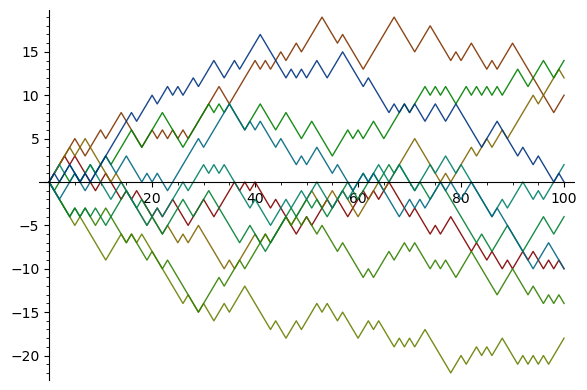
Brownian motion can be thought of as a mathematical limit of a random walk. In particular, consider a 1-dimensional process in which the state (a number) changes by a fixed positive or negative increment with equal probability. The figure below shows a 10 realizations of such a process, for 100 steps, in each case starting at 0 and with increments 1 and -1.

If we decrease the time taken for each step by a factor of $k$, the variance of the total of all steps taken in a fixed time period will increase by a factor of $k$. So if we want the standard deviation of the process to stay constant as we decrease this interval, the standard deviation of each step needs to be decreased by $\sqrt{k}$. The result is the Brownian motion stochastic process (sometimes called the Weiner process in honor of Norbert Wiener), which starting from $x_0=0$ has the probability distribution:

Stochastic differential equations are usually written in terms of increments rather than derivatives, since they are not usually differentiable functions (they are best defined as integral equations). For a SDE of the form

we can simulate an initial value problem's solution using the Euler-Marayama method, which generalizes the usual Euler's method. If $x(t_0) = x_0$, then for a timestep $k = \Delta t$ we approximate using

where $w_i$ is a random sample drawn from a normal distribution with mean $0$ and variance $1$.

The key point is the scaling of the stochastic component by $\sqrt{k}$, rather than $k$.

Additional Exercises

1-3. For the first three differential equations find the equilibria and determine their stability. Then sketch some of the typical trajectories starting near each equilibrium.

1. $y' = y - 5$

2. $y' = y^2 - 3y$

3. $y' = (y-1)^2$

   
   

4. Consider a fish population that would change according to the logistic equation, $P' = k P ( M - P)$ if it were undisturbed. Suppose that these fish will be removed at a rate $hP$ for some $h \ge 0$. If $k=1$ and $M=1000$, find the value of $h$ that will maximize the number of removed fish at a stable equilibrium population.

5. Use all three of the numerical methods (Euler, Improved Euler, and 4th-order Runge-Kutta) to find the value of $y(1)$ to four digits of accuracy using the smallest possible number of steps if $y' = x y - y^3$ and $y(0) = 1$. How many steps are necessary for each method? For this question you can use the functions from the lab 3 to do the computations.

6. You jump out of an airplane at a height of 3000 meters. After 20 seconds, you open your parachute. Assume a linear air resistance with a drag acceleration of $rv$ where $r = 0.15$ without that parachute and $r = 1.5$ with the parachute. How long does it take to reach the ground?

7. Suppose that the drag acceleration was exactly proportional to the square of the velocity, so $\displaystyle \frac{dv}{dt} = - k v^2$. If there were no other forces involved, and the intial velocity and position were $v(0)= v_0 > 0$, $x(0) = x_0$, how far would a particle travel before coming to rest?

Notes

Notes: (Local storage in a cookie) Add

License

This work (text, mathematical images, and javascript applets) is licensed under a Creative Commons Attribution-NonCommercial-ShareAlike 4.0 International License. Biographical images are from Wikipedia and have their own (similar) licenses.