Vector Spaces

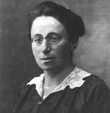
The idea of a vector arose from mathematical representations of 2- and 3-dimensional positions, velocities, accelerations, forces, momenta and other quantities in physical models. This remains one of the primary contexts in which we usually first learn about vectors. However, starting in the late 19th century mathematicians (and physicists, chemists, and engineers) found it was useful to abstract the mathematical essence of these vectors into a more general structure. Hermann Grassman laid many of the foundations for linear algebra in his 1844 book "Die Lineale Ausdehnungslehre", but it was somewhat ahead of its time, and it wasn't until 1888 that Peano wrote an explicit definition of vector spaces. The further development of abstract algebraic structures has exploded since then, with some of the other early steps being taken by Arthur Cayley, Charles Sanders Pierce, David Hilbert, and Emmy Noether.

It can be very difficult to grasp such abstract structures. The most important thing to remember is that these abstract structures were directly inspired by particular examples, and it is crucial to repeatedly consider them through concrete (or at least relatively concrete) examples.

Fields

In this section we will present the basic definitions and ideas for an abstract vector space over a field.

Vector spaces are sets (collections of items, or elements) whose elements (the vectors) can be added together, or scaled by some scalar quantity. The scalar quantities belong to a field; a field is a kind of number system. The idea of a field is to generalize the operations of arithmetic. Let's start with some examples of fields, and examples of things that are not fields, before looking at their formal properties.

The most familiar field, and the inspiration for all of the others, is the set of rational numbers. We will denote this field by $\mathbb{Q}$. The elements of $\mathbb{Q}$ are ratios of integers, such as $\frac{3}{2}$ or $\frac{-2}{5}$ or $\frac{7}{1} = 7$ (technical caveat: the denominator cannot be 0). The field operations are the usual addition, subtraction, multiplication, and division that we learn as children.

One property of the rational numbers that we want every field to have is that every non-zero rational has a multiplicative inverse: if $a \in \mathbb{Q}$ and $a \neq 0$ then there is a rational number $b$ such that $a b = 1$. The integers $\mathbb{Z} = \{ \ldots, -3, -2, -1, 0, 1, 2, 3, \ldots \}$, which are a subset of $\mathbb{Q}$, are not a field because their inverses are not always integers (e.g. the inverse of $2$ is $\frac{1}{2}$, which is not an integer).

Another property of the rational numbers is that their multiplication is commutative: if $a$ and $b$ are in $\mathbb{Q}$ then $a b = b a$. Because matrix multipication is not commutative, most subsets of matrices such as the set of $2$ by $2$ matrices with rational entries are not fields.

In elementary school you may have learned some of the field properties of the rationals. I am not sure why people are taught this in elementary school, because it only makes sense in the context of general fields. If $a$, $b$, and $c$ are arbitrary rational numbers, we can state the commonly taught properties as:

1) Addition is commutative: $a + b = b + a$

2) Multiplication is commutative: $a b = b a$

3) Addition is associative: $(a + b) + c = a + (b + c)$

4) Multiplication is associative: $(a b) c = a (b c)$

5) Addition and multiplication are distributive: $a(b + c) = a b + a c$

We also want every field to have elements that are analogous to $0$ and $1$; we usually write them as $0$ and $1$:

6) There is an additive identity element, denoted $0$ (or $O$): $0 + a = a$

7) There is a multiplicative identity element, denoted $1$ (or $I$): $1 a = a$

Finally we want nonzero field elements to be invertible:

8) Every $a$ has an additive inverse $-a$: $a + (-a) = 0$

9) Every $a \neq 0$ has a multiplicative inverse $a^{-1}$: $a a^{-1} = 1$.

We can think of subtraction in terms of inverses as a special case of addition: $a - b = a + (-b)$, and division as a multiplication: $a/b = a b^{-1}$.

In this text we mainly use two fields: the real numbers $\mathbb{R}$ and the complex numbers $\mathbb{C}$. But there are other applications, such as cryptography, where more exotic fields are useful. Let's look at one example of different field.

Example: The Field of Four Elements

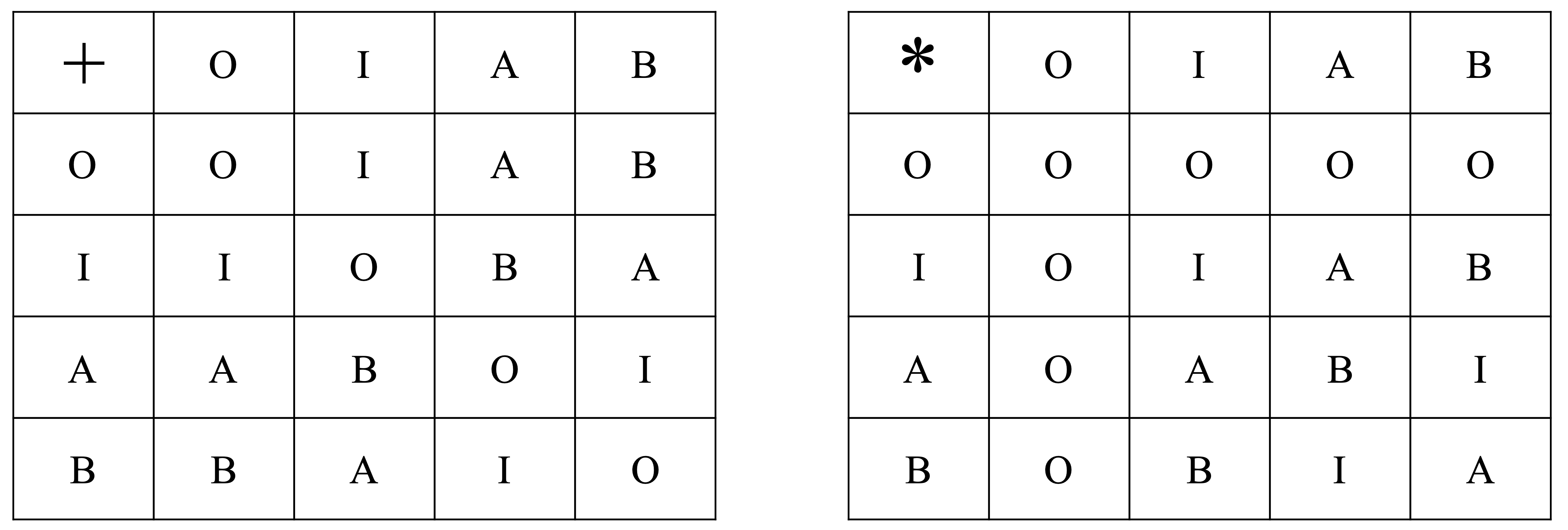
There are finite fields, which as the name suggests have only a finite number of elements. It is not too hard to prove that any finite field must have a prime power number of elements; it is somewhat harder to show that for every prime power there is a field with that number of elements. For example, since $4 = 2^2$ is a prime power, there is a field with 4 elements. It is sometimes denoted by $F_4$. It must have a zero, let's denote that by $O$, and a multiplicative identity, which we will denote by $I$. The other two elements we will call $A$ and $B$.

We know that $A + O = A$, and $B + O = B$, and $A I + A$, and $B I = B$. But what is $A + A$, or $AB$ equal to? To be consistent with all of the field rules we are lead to a unique answer.

Coordinate Vector Spaces

Before formally defining vector spaces it may help to consider the inspiration for them, coordinate vector spaces. The main examples of these are $\mathbb{R}^2$ and $\mathbb{R}^3$, the plane and real 3-D space considered as vector spaces. The vectors are simply lists of coordinates, which can be considered as either $1 \times n$ matrices (row vectors) or $n \times 1$ matrices (column vectors). The vector operations are then just matrix scalar multiplication and addition.

Abstract Vector Spaces

An abstract vector space is any set $V$ on which we can define a scalar multiplication by a field (call it $F$) and an addition operation between vectors which have the same algebraic properties as the coordinate vector space operations. In terms of arbitrary vectors $u, v, w \in V$ and scalars $s,t \in F$, these are:

1) $u + v = v + u$ (addition of vectors is commutative)

2) $u + (v + w) = (u + v) + w$ (addition of vectors is associative)

3) $0 + u = u$ (there is a zero vector in $V$ that is the identity element for vector addition)

4) $u + (-u) = 0$ (for every vector there is an additive inverse vector in $V$)

5) $s(t u) = (st) u$ (the field multiplication is associative with respect to scalar multiplication)

6) $1u = u$ (multiplying a vector by the scalar field identity also acts by identity)

7) $s(u + v) = su + sv$ (scalar multiplication distributes over vector addition)

8) $(s + t)u = su + tu$ (scalar multiplication distributes over vector addition, in both senses)

Examples of Vector Spaces

The coordinate vector spaces are the main example, but there are many other vector spaces. Here are a few examples:

1) $m \times n$ matrices with real entries; as a vector space we ignore the matrix-matrix multiplication possibilities, and just consider the scalar multiplication and addition.

2) The set of functions $e^{kt}$ where $k$ is a real number and $t$ is an independent variable. The scalar multiplication is just the usual multiplication by constants, and addition is also just usual addition of functions.

3) The set of polynomials of degree at most $d$ in a variable $x$, $P_d$, is a vector space. For example, if $d=3$ then $P_3$ is the set of polynomials of the form $a_0 + a_1 x + a_2 x^2 + a_3 x^3$ where the $a_i$ are real constants. The vector operations are just usual addition and scalar multiplication.

4) The set of solutions to the differential equation $\frac{d^2 y}{dx^2} - xy = 0$ forms a vector space over the real numbers. If $y_1$ and $y_2$ are solutions to that ODE, then so is $c_1 y_1 + c_2 y_2$ for any choice of real numbers $c_1$ and $c_2$.

Vector Subspaces

A subset $W \subset V$ of a vector space $V$ is a vector subspace (often we just say subspace) if it is a self-contained vector space in its own right. This means that if we start with two elements $w_1$ and $w_2$ in $W$, any vector arising from the vector space operations on them should still be in $W$; in other words, for any scalars $c_1$ and $c_2$, $c_1 w_1 + c_2 w_2 \in W$. This is called closure under the vector space operations.

Examples of Vector Subspaces

The main examples of subspaces are:

1) In $\mathbb{R}^2$ there are only three kinds of subspaces: the whole plane $\mathbb{R}^2$ itself, the origin $\{(0,0)\}$, and lines through the origin. The first example is somewhat silly, so often we want to restrict to proper subspaces, which are vector subspaces that are strictly smaller than the ambient vector space.

2) In real space ($\mathbb{R}^3$) the only proper subspaces are the $\{(0,0,0)\}$, lines through the origin, and planes through the origin. Any other subset will fail to be a subspace by some sort of failure of the closure condition.

3) Solution subspaces. Any homogeneous linear system has a solution set that is a vector subspace of a coordinate space. For example, the set of solutions to

is a vector subspace of $\mathbb{R}^4$.

Example: The square is not a subspace

No bounded subset of the plane is a subspace; we will look at the concrete example of the square

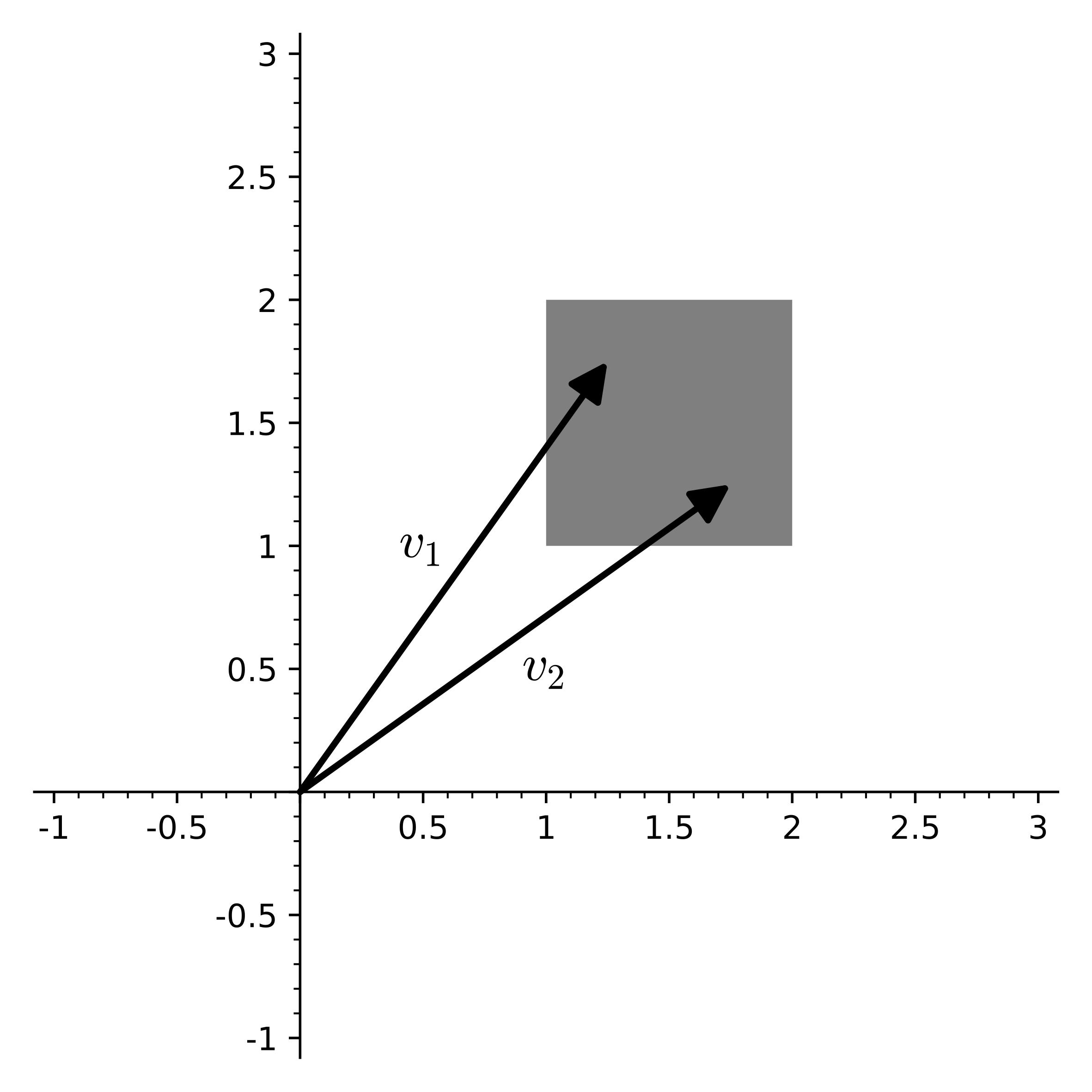
Two vectors in $S$, $v_1 = (1.25,1.75)$ and $v_2 = (1.75,1.25)$, are shown in the picture. To be a vector subspace, any scalar multiple of $v_1$ or $v_2$ would have to still be in $S$. But the multiple $0 v_1 = (0,0)$ is not in $S$, so it is not a vector subspace. Any linear combination of $v_1$ and $v_2$ would also have to stay in $S$, but this also fails in many cases, such as $v_1 + v_2 = (3,3) \notin S$.

Exercises

1. Is the subset $W = \{(x,y) \ | \ y \ge 0 \} \subset \mathbb{R}^2$ a vector subspace of $\mathbb{R}^2$? Explain why or why not.

2. Is the subset $W = \{(x,y) \ | \ y = 0 \text{ or } x = 0\} \subset \mathbb{R}^2$ a vector subspace of $\mathbb{R}^2$? Explain why or why not.

3. Is the set of two-by-two skew-symmetric matrices ($A^T = -A$) a vector subspace of the set of all two-by-two matrices with real entries?

Linear dependence and independence

It is often necessary to know how different vectors are related; in particular whether or not (and how) we can write some vectors in terms of others. For example, colors on computer screens are often represented as triplets of Red, Green, and Blue (RGB) values. In some applications we might want to use a limited color palette, and perhaps would want to know if a particular color such as $v_1 = (35, 85, 110)$ is a combination of two other colors such as $v_2 = (10,5,40)$ and $v_3 = (5,25,10)$. In this case the answer is yes, $v_1 = 2v_2 + 3v_3$. If we move all of the vectors to one side of the equation, this gives us the linear dependence relation:

In general if we have a set of vectors $\{v_1, v_2, \ldots, v_n\}$ they are defined to be linearly dependent if there exist numbers (scalars, or field elements) $c_1, c_2, \ldots, c_n$ which are not all zero such that

In our example, $c_1 = -1$, $c_2 = 2$, and $c_3 = 3$ was one choice of scalars that shows that those vectors $v_1$, $v_2$, and $v_3$ are not independent.

Conversely if there is no such choice of $c_i$ which are not all zero, the vectors are linearly independent. A simple but very important set of examples are the standard bases for $\mathbb{R}^n$. For $\mathbb{R}^2$, the standard basis is $v_1 = (1,0)$ and $v_2 = (0,1)$. These are linearly independent since the requirement that

is equivalent to the two scalar equations $c_1 = 0$ and $c_2 = 0$, but we must have at least one nonzero $c_i$ for the vectors to be linearly dependent.

We can systematically determine if a set of vectors is linearly dependent by writing the dependence condition as a linear system of equations and row-reducing its coefficient matrix. Lets look at an example.

Span of a set of vectors

Closely related to the notions of linear dependence and independence is the span of a set of vectors, which is the subspace of all linear combinations of those vectors.

For example, the span of the single vector $(1,1)$ in the $(x,y)$ plane is the line $c_1 (1,1) = (c_1, c_1)$, which can also be described as the line $y=x$.

The span of the set $\{(0,0),(1,0),(-2,0)\}$ in the $(x,y)$ plane is just the $x$-axis; we only need either of the last two vectors in the set to generate the same span.

Example: Linear Dependence Determination

Are the vectors $v_1 = \left ( \begin{array}{c} -1 \\ 2 \\ 0 \\ 1 \end{array} \right )$, $v_2 = \left ( \begin{array}{c} 2 \\ 0 \\ 3 \\ -3 \end{array} \right )$, $v_3 = \left ( \begin{array}{c} 1 \\ -1 \\ 1 \\ -1 \end{array} \right )$, $v_4 = \left ( \begin{array}{c} 3 \\ 5 \\ 8 \\ -6 \end{array} \right )$ linear dependent or independent?

We want to analyze the set of $c_i$ such that $c_1 v_1 + c_2 v_2 + c_3 v_3 + c_4 v_4 = 0$. As a matrix-vector system this is:

Because this is a homogeneous system (the right-hand side is the zero vector) we only need to row reduce the coefficient matrix (none of the row operations would affect the entries of the zero vector). If the row-reduced echelon form of the coefficient matrix has fewer than four pivots, one of the $c_i$ is a free variable and we can choose it to be nonzero to obtain a linear dependence.

Here is one sequence of row operations that transform the coefficient matrix to its rref:

The reduced row echelon form only has three pivots, and $c_4$ is a free variable. If we choose $c_4 = 1$, then the rref rows also show us that we must have $c_1 = -2$, $c_2 = -3$, and $c_3 = 1$, and the dependence relation is

Another way to interpret this is that we write $v_4$ in terms of the other vectors:

Basis and Dimension

It is often extremely useful to have an efficient representation of a vector space in terms of some fundamental vectors that generate the space. The most common structure for this is a basis for a vector space, which has the following definition:

Definition: a basis for a vector space $V$ is a set of linearly independent vectors whose span is $V$.

There is a tension between the independence of the vectors, which forces the basis set to be small, and the requirement of spanning the space, which forces the basis to have a minimal size. It turns out that while there are usually many different bases for a given vector space, they always have the same number of elements.

Definition: the dimension of a vector space is the number of vectors in any basis of that space.

Exercises:

1. $a$ Are the vectors $v_1 = \left ( \begin{array}{r} 1 \\-1 \\ 0 \\ 2 \end{array} \right )$, $v_2 = \left ( \begin{array}{r} 2 \\ 0 \\ -2 \\ 1 \end{array} \right )$, and $v_3 = \left ( \begin{array}{r} 0 \\ 1 \\ -1 \\ -\frac{3}{2} \end{array} \right )$ linearly independent or dependent?

   $b$ If they are linearly dependent, find constants $c_1, c_2, c_3$, not all zero, such that $c_1 v_1 + c_2 v_2 + c_3 v_3 = 0$.

2. Let $W = \text{span}(\{ v_1, v_2, v_3\})$. Find a basis for $W$, and determine its dimension.

Example: Bezier basis for polynomial spaces

Spaces of polynomials are a good example of vector spaces that are somewhat different from standard coordinate vector spaces. Let us denote the space of polynomials with real coefficients and a maximum degree of $n$ by $\mathcal{P}_n$. For example, $\mathcal{P}_3$ is the space of cubic polynomials. We most often write a cubic in terms of the power basis $(1,x,x^2,x^3)$ - so if $p \in \mathcal{P}_3$ we write

This choice of (ordered) basis gives us a way to associate polynomials with coordinate vectors:

However, $\mathcal{P}_3$ is not the same as $\mathbb{R}^4$, and although the power basis may seem natural it is not the only choice of basis. In fact for many practical purposes the power basis is a bad choice, and it is better to use a different basis. In graphic design and computer graphics many shapes (including the letters of this document) are described with Bezier curves, which for cubics use the alternative basis

The Bezier basis leads to a different way of associating polynomials to coordinate vectors. For example, the cubic polynomial $1 - 6x + 12x^2 - 8x^3$ in the Bezier basis looks like this:

These choices of association - the isomorphisms between the vector spaces - can be related by a matrix. For the above example, we can relate the representation in the standard basis to the Bezier basis by expanding the Bezier basis polynomials:

giving us the change of basis matrix

The inverse of $B$ is

We can use these to go back and forth between different representations of polynomials. For example, going from the power basis representation of $1 - 6x + 12x^2 - 8x^3$, which is $(1,-6,12,8)$, to the Bezier basis we use $B^{-1}$:

Solution sets as bases

One of the main reasons we care about the idea of vector subspaces is that they arise naturally as the sets of solutions to homogeneous linear systems - for both algebraic and differential equations. For nonhomogeneous systems the solution set is not a subspace, but it can be described as a translated (shifted) copy of the corresponding homogeneous solution subspace. Let's look at an example.

Example: Subspace structure of solution sets

We will describe the solutions $x=(x_1,x_2,x_3,x_4)^T$ to the system

in terms of its vector space structure.

Most of the work in analyzing this kind of problem is the computation of the row reduced echelon form (rref) of the augemented coefficent matrix. In this case that is not too bad:

This tells us that $x_1$ and $x_3$ are the pivot variables, because the pivots of the rref are in the 1st and 3rd columns. We can write them in terms of the other variables - the free variables - $x_2$ and $x_4$. The first row is equivalent to $x_1 + 2 x_2 + 2x_4 = -1$, or $x_1 = -2 x_2 - 2x_4 - 1$. Likewise, the second row is equivalent to $x_3 = -x_4 + 2$. We can rephrase this in vector form - the solution $x$ to the system in terms of the free variables is:

This shows that any solution $x$ can be written as an element of the homogeneous solution subspace,

plus a shift $x_p = (-1,0,0,2)^T$,

Exercise

1. Find a basis for the subspace defined by the following equations for $(x_1,x_2,x_3,x_4,x_5) \in \mathbb{R}^5$. Your answer should be a set of five-dimensional vectors.

   $$\begin{split} 2x_1 + x_3 - 2x_4 - 2x_5 & = 0 \\ x_1 + 2x_3 - x_4 + 2x_5 & = 0 \\ -3x_1 - 4x_3 + 3x_4 - 2x_5 & = 0 \end{split}$$

Inner products and angles

A vector space $V$ over a field $F$ can be given some extra geometric structure (lengths and angles) by choosing an inner product, which is a scalar function of two vectors in $V$ satisfying some axioms that are inspired by the usual Euclidean dot product of real vectors.

There are several notations used for inner products; we will use $<u, v>$ to denote the inner product between vectors $u$ and $v$.

The standard inner product for real coordinate vector spaces $\mathbb{R}^n$ is

where the vectors are usually thought of as column vectors ($n$ by $1$ matrices).

Inspired by the standard product we demand that any abstract inner product on a vector space have the properties:

1) Scalar linearity: if $s$ is a scalar, then $<s u, v> = s <u, v>$

2) Vector linearity: if $u$, $v$, and $w$ are vectors in $V$, then $<u + v, w> = <u,w> + <v,w>$

3) Hermitian symmetry: $<u,v> = \overline{<v,u>}$; this is just the symmetry condition $<u,v> = <v,u>$ for real vector spaces.

4) Positive definiteness: $<u,u> \ \ge 0$ and $<u,u> = 0$ only if $u$ is the zero vector.

We can define the length of a vector by

and the angle $\theta$ between two vectors $u$ and $v$ is defined by

The Rank-Nullity Theorem

One of the most important unifying theorems about linear transformations of finite-dimensional vector spaces is the rank nullity theorem. We will phrase this theorem in terms of (real) matrices, although it applies more generally.

Suppose that $A$ is a $m$ by $n$ matrix. Consider the linear transformation $f(x) = Ax$, which maps input vectors from $\mathbb{R}^n$ to output (range) vectors in $\mathbb{R}^m$. Mathematicians often indicate this as:

There are two important subspaces associated with this map:

The kernel, or nullspace, of $A$ (really of $f$, but we tend to refer to the function through the matrix) is the subspace of $\mathbb{R}^n$ that is sent to zero by $Ax$. It is a subspace since if $Ax = 0$ and $Ay = 0$, then for scalars $c_1$ and $c_2$

The kernel is usually denoted by either $ker(A)$ or $N(A)$.

The range of $A$ (again, really the range of the function $f=Ax$), also called the column space of $A$, is the subspace of all image vectors under the map $f$. This is the same as the span of the columns of $A$, since if we write $A$ as $n$ columns $A = (a_1|a_2|\ldots|a_n)$ then

The range of $A$ is denoted by $R(A)$ (or in some texts as $Col(A)$).

The rank-nullity theorem relates the dimensions of these for any matrix:

The dimension of the range, $dim(R(A))$, is also called the rank of $A$, and the dimension of the nullspace, $dim(N(A))$, is also called the nullity of $A$.

Additional Exercises

1. Is the subset $W = \{(x,y,z) \ | \ y \ge 0 \} \subset \mathbb{R}^3$ a vector subspace of $\mathbb{R}^3$? Explain why or why not.

2. Is the subset $W = \{(x,y,z) \ | \ y = 0 \} \subset \mathbb{R}^3$ a vector subspace of $\mathbb{R}^3$? Explain why or why not.

3. If $W$ is the subset of all vectors $(x,y)$ in $\mathbb{R}^2$ such that $|x| = |y|$, is $W$ a vector subspace or not?

4. Suppose that $x_0$ is a solution to the equation $Ax=b$ (where $A$ is a matrix and $x$ and $b$ are vectors). Show that $x$ is a solution to $Ax = b$ if and only if $y = x - x_0$ is a solution to the system $Ay = 0$.

5. Determine whether the vectors $v_1 = (3,0,1,2)$, $v_2 = (1,-1,0,1)$, and $v_3 = (4,2,2,2)$ are linearly independent or dependent. If they are linearly dependent, find a non-trivial combination of them that adds up to the zero vector.

6. Find a basis for the subspace of $\mathbb{R}^3$ given by $x - 2y + 7z = 0$.

7. Find a basis for the subspace of $\mathbb{R}^3$ given by $x = z$.

8. Find a basis for the subspace of all vectors $(x_1,x_2,x_3,x_4)$ in $\mathbb{R}^4$ such that $x_1 + x_2 = x_3 + x_4$.

   The following two questions are about subsets of the set of real-valued functions of the real line. We will call this set $\mathcal{F}$; it is a vector space over the real numbers.

9. Is the subset of $\mathcal{F}$ with the property that $f(0) = 0$ a vector space?

10. Is the subset of $\mathcal{F}$ with the property that $f(-x) = -f(x)$ for all $x$ a vector space?

Notes

Notes: (Local storage in a cookie) Add

License

This work (text, mathematical images, and javascript applets) is licensed under a Creative Commons Attribution-NonCommercial-ShareAlike 4.0 International License. Biographical images are from Wikipedia and have their own (similar) licenses.