Linear systems and Matrices

Linear Equations

We begin our coverage of linear algebra with the topic of linear algebraic equations. Sometimes people get the mistaken impression that this is the primary subject of linear algebra, but it is merely the historically (and pedagogically) first case in which linear algebra was needed. As an analogy, linear equations are to linear algebra as the study of batteries is to electrical engineering.

Let us briefly review the 2-dimensional case, in which we have a system of equations:

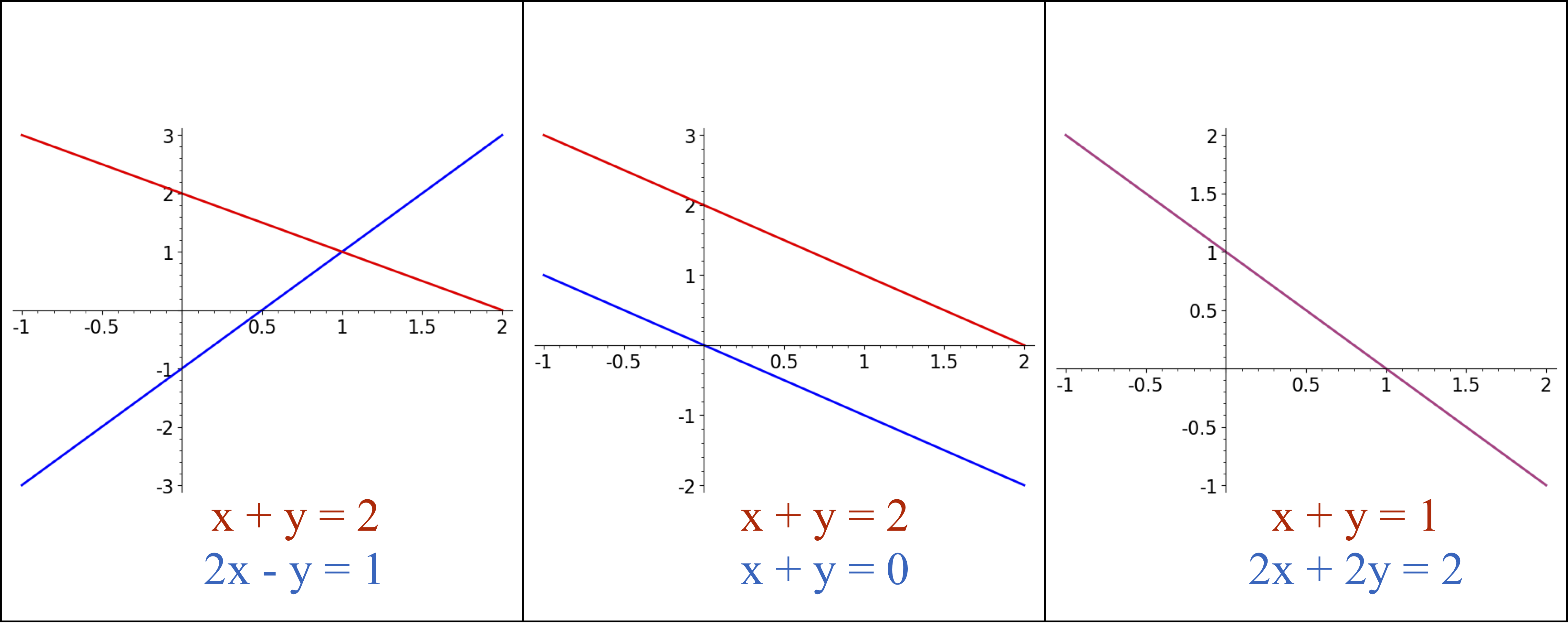
where the $a_{i,j}$ and $b_i$ are fixed parameters and we want to characterize the solutions $(x,y)$. Geometrically this system can be interpreted as the intersection of two lines in the $(x,y)$ plane. There are three possiblities for the solution set: (1) a unique point of intersection, (2) no points of intersection, and (3) infinitely many points of intersection (when the two lines are the same).

To solve a 2D linear system, you may have learned to solve for one of the variables, e.g. $y$, in terms of the other, and then substitute that into the second equation. For larger systems it is more efficient to use linear combinations of equations to eliminate variables. Let us look at an example to illustrate this idea.

---

Example: 3x3 linear system

Find all solutions to the linear system

Note that in this 3-dimensional example we can interpret the system as requiring a common point of intersection for three planes.

We begin by eliminating $x$ from equations (2) and (3) by adding a multiple of the first equation to them. If we add $-4$ times equation (1) to equation (2), we get

and similarly after adding $-7$ times equation (1) to equation (3) we get

We can simplify these two new equations by dividing by $-3$ and $-6$, respectively, which results in the new common equation:

This is unusual; for a random set of three linear equations we would not arrive at the same equation after analogous steps. The original system is equivalent to a pair of linear equations in three variables, which is geometrically the intersection of two (rather than 3) planes. So we have an entire line of solutions. If we use the $z$ coordinate to parameterize this line, we need to solve for $x$ and $y$ in terms of $z$. Before doing this we further simplify the system by using the equation (4) to eliminate $y$ from equation (1) by adding -2 times equation (4) to equation (1), yielding the following system which is equivalent to the original one:

which we can solve for $x$ and $y$ in terms of z:

so the line of solutions is of the form

---

Exercise:

1. Find all the solutions to the equations

Augmented coefficient matrices

For larger linear systems it becomes cumbersome to manipulate the equations while eliminating variables. The bookkeeping can be simplified and systematized by using augmented coefficient matrices. Let's look at an example

---

Example: augmented coefficient matrix

The system of equations

can be represented by the equivalent augmented coefficient matrix:

The 3 by 3 submatrix on the left-hand side is the coefficient matrix of the system - i.e. the coefficients of the variables in each equation, while the right-hand column represents the constants in the linear equations.

---

Elementary Row Operations and Echelon Forms

To solve a linear system we will eliminate each variable from the equations as much as possible, starting with the first (left-most) variable. There are three types of operations we can perform on the equations (or equivalently on the augmented coefficient matrix) which are reversible and which do not change the solution set of the equations:

1) Row swaps (interchanging equations)

It does not matter what order we write our equations in, so we are free to interchange them. For the augmented coefficient matrix this corresponds to interchanging rows. The elementary operation is to only swap two rows; any other permutation of rows can be built up from these row swaps. In our previous example we may wish to interchange rows 1 and 2, which we write as

(The "S" is an abbreviation for "swap".)

2) Row rescaling.

We can multiply an equation by a nonzero constant without changing its solutions. Equivalently, we can multiply a row in the augmented coefficient matrix by any nonzero constant, for example:

3) Adding a multiple of one row to another

The most powerful operation we can perform is to add a multiple of one equation (row) to another. This is the primary way we eliminate variables from some equations. In our running example, if we want to eliminate $x$ (corresponding to the first column of the matrix) as much as possible we can subtract two times the first row from the second.

IMPORTANT NOTE: The way we write the third row operation type is not commutative: $\xrightarrow{-R_1 + R_2}$ means something very different from $\xrightarrow{R_2 - R_1}$. The first means: subtract row 1 from row 2. The second is not an elementary operation, but it is a combination of two elementary operations: first reverse row 1, and then add row 2 to row 1.

The reduced row echelon form (rref)

Using the elementary row operations we can simplify matrices. For many purposes, including solving linear systems of equations, it is helpful to reduce the matrix to a standard form, called the reduced row echelon form, also abbreviated as rref. The main idea is to work left-to-right, simplifying each column as much as possible before working on the next. The precise definition of the reduced row echelon form is:

1. Any all-zero rows are below non-zero rows

2. The first (leftmost) nonzero entry in each row, called a pivot, is equal to 1.

3. Everything above and below a pivot (in the same column) is zero.

4. Each pivot is to the right of the pivots above it.

---

Example

We will use elementary row operations to find all of the solutions to the linear system

(For larger linear systems it becomes convenient to use indexed variables, since otherwise we run out of letters. We will often use $x_1$, $x_2$, et cetera instead of $x$, $y$, and $z$.)

The augmented coefficient matrix for this system is

Before doing the row operations, let's pause a moment and think about what we can expect to happen. We have 3 linear equations in 4 unknowns; usually if we have more unknowns than equations the system is underdetermined, and there will be infinitely many solutions. This problem is analogous to the intersection of two planes in 3D (two linear equations in three unknowns), for which usually the planes will intersect in a line. Just as it is possible to have two parallel planes which do not intersect, this problem could have no solutions, but that is a delicate state that is unlikely for a 'random' problem.

Now we will compute the reduced row echelon form of the augmented coefficient matrix. We can use the first row to eliminate the other entries of the first column:

A quirk of this matrix is that we have also reduced the second column (usually that won't be the case), so we can move onto reducing the third column.

Finally we clean up the fourth column using the pivot at position $(3,4)$:

The rref gives us the equivalent simpler system

Variables corresponding to columns with pivots are called pivot variables, and any other variables are called free variables. We can write all of the solutions in terms of the free variables. In this case, that just amounts to moving the only free variable, $x_2$, over to the other side, so all solutions can be written as: $x_1 = -x_2 + 1/7$, $x_3 = 3/7$, and $x_4 = 4/7$, where we can choose any $x_2$ value.

---

Basic Matrix Algebra

So far we've used matrices as book-keeping devices for solving linear equations, but it turns out to be very useful to consider them as mathematical objects in their own right.

We give matrices an algebraic structure with three fundamental operations: addition, matrix-matrix multiplication, and scalar-matrix multiplication. In context, we will refer to the last two operations more succinctly as matrix multiplication and scalar multiplication.

The addition of matrices is only defined for matrices of the same shape: if $A$ is a $m$ by $n$ matrix ($m$ rows and $n$ columns) then it can only be added to other $m$ by $n$ matrices. The definition of matrix addition is very simple: we simply add the elements component-wise. If $A$ and $B$ are $m$ by $n$ matrices, then the sum $C = A + B$ is a $m$ by $n$ matrix whose $(i,j)$ entry $C_{i,j}$ is $A_{i,j} + B_{i,j}$.

For example,

Scalar multiplication is also fairly simple: if we multiply a matrix by a scalar, all of the entries of the matrix are multiplied by that scalar. For example:

In general, if $A$ is a $m$ by $n$ matrix and $k$ is a scalar (e.g. a real or complex number), then $kA$ is also a $m$ by $n$ matrix with entries $k A_{i,j}$.

The multiplication of matrices is much less intuitive. If $A$ is a $m$ by $n$ matrix, it can multiply a $n$ by $p$ matrix $B$ from the left: $C = AB$, and the result $C$ will be a $m$ by $p$ matrix. The entries of this resulting matrix are defined as

Matrix multiplication is not commutative: $AB$ does not have to equal $BA$, and both products are not always defined at all. Let us look at some examples.

---

Example: Matrix multiplication

If

(a 3 by 3 matrix) and

(a 3 by 2 matrix), then $BA$ is not defined, and

---

Why multiply this way?

Matrix multiplication is not commutative (i.e. $AB \neq BA$ in general) and is considerably more complicated than the more natural-seeming componentwise multiplication we could use. Why do we define it this way?

The reason is that we use matrices to realize linear transformations, and if we compose linear transformations then the composite can be represented as a multiplication of the individual matrices. Let us look at the smallest example that illustrates this idea - 2 by 2 matrices.

Suppose that we have quantities $y_1$, $y_2$ that are linear functions of $x_1$ and $x_2$:

(The $a_{i,j}$ are constants.)

Furthermore, we also have $z_1$ and $z_2$ that are linear functions of $y_1$ and $y_2$:

If we define the coefficient matrices

and we package our variables into two by one matrices (column vectors) $x=\left ( \begin{array}{r} x_1 \\ x_2 \end{array} \right)$, $y=\left ( \begin{array}{r} y_1 \\ y_2 \end{array}\right)$, $z=\left ( \begin{array}{r} z_1 \\ z_2 \end{array}\right)$, then the definition of matrix multiplication lets us write everything above as

where

---

Example: Dangers of matrix algebra

This example illustrates some of the crucial differences between matrix algebra and the more familiar algebra of real and complex scalars. Consider the matrices

and

We can compute the products $A B$ and $A C$:

So $A B = A C$, and therefore $A(B -C) = 0$. Note however that we cannot divide matrices, and we cannot conclude that either $A = 0$ or $B=C$ (neither is true here).

---

Additive and multiplicative identities

There is a family of matrices which act as the number 1 does for scalars - i.e. they are the multiplicative identity in matrix algebra. They are square matrices, $n$ by $n$, which have diagonal elements equal to 1 and the off-diagonal elements are zero. For example, the three by three identity matrix is

Usually the size of the identity matrix is clear from context, and so they are each just denoted as $I$.

The zero matrix (the matrix of all zeros, for each dimension of matrix) is the additive identity. It is common to denote the zero matrix by the usual scalar 0; its dimension can be inferred by context.

The transpose

The transpose $A^T$ of a matrix $A$ is the matrix formed by using the rows of $A$ as columns, i.e. $(A^T)_{i,j} = A_{j,i}$. For example, if $A = \left(\begin{array}{rr} 1 & 2 \\ 3 & 4 \end{array}\right)$ then $A^T = \left(\begin{array}{rr} 1 & 3 \\ 2 & 4 \end{array}\right)$.

---

Exercises

Compute the rref (reduced row echelon form) of the following three matrices. The rref is defined by the properties:

• Any all-zero rows are below non-zero rows

• The first (leftmost) nonzero entry in each row, called a pivot, is equal to 1.

• Everything above and below a pivot (in the same column) is zero.

• Each pivot is to the right of the pivots above it.

• $\left ( \begin{array}{rrrr} 2 & 2 & 2 & 2 \\ 1 & 1 & 1 & 1 \\ 0 & 1 & 2 & 3 \\ 0 & -1 & -2 & -3\end{array} \right )$

• $\left ( \begin{array}{ccc} a & a & b \\ b & b & c \\ 0 & 0 & -1 \end{array} \right )$ where $a$, $b$, and $c$ are distinct and nonzero.

• $\left ( \begin{array}{rrrr} 0 & 0 & 2 & 1 \\ 0 & 0 & 1 & 2 \end{array} \right )$

• If $B = \left ( \begin{array}{ccc} 1 & 2 & 3 \end{array} \right )$ and $C = \left ( \begin{array}{r} -2 \\ -2 \\ 2 \end{array} \right )$, compute both $BC$ and $CB$.

• Describe all two by two matrices $A = \left ( \begin{array}{cc} a & b \\ c & d \end{array} \right )$ which commute with $B = \left ( \begin{array}{cc} 1 & 2 \\ 3 & 4 \end{array} \right )$ (i.e. $AB=BA$).

• If $B = \left ( \begin{array}{rr} 2 & 1 \\ 3 & 2 \end{array} \right )$, find a matrix $A = \left ( \begin{array}{rr} a & b \\ c & d \end{array} \right )$ such that

  $$A B = \left ( \begin{array}{rr} 2 & 0 \\ 0 & 2 \end{array} \right )$$

  by equating the individual entries on both sides of the equation.

• For $A = \left ( \begin{array}{rr} 1 & -2 \\ -2 & 4 \end{array} \right )$, find a non-zero matrix $B = \left ( \begin{array}{rr} a & b \\ c & d \end{array} \right )$ such that

  $$A B = \left ( \begin{array}{rr} 0 & 0 \\ 0 & 0 \end{array} \right )$$

---

Matrix inverses and elementary matrices

In ordinary arithmetic multiplication and division are usually thought of as inverse operations. We can also view division as a form of multiplication (a source of some confusion I think for people learning about fractions); for example the expression $\frac{3}{4}$ is both $3$ divided by $4$, and $3$ times the inverse of $4$. Within the real number system, only zero lacks a multiplicative inverse.

For matrices we avoid ever using the notation of division. This is partially because of the non-commutativity of matrix algebra, which makes it awkward to show exactly where we want to divide. It is also because many matrices are not invertible:

• Definition: A square matrix $A$ is invertible if there exists a matrix $B$ such that $BA = AB = I$, where $I$ is the identity matrix with the same dimensions as $A$.

If a matrix $A$ has an inverse, we can denote it by $A^{-1}$. This is unambiguous, because matrix inverses are unique. Suppose that $B$ and $C$ are both inverses of a matrix $A$. Then $B = IB = CAB = CI = C$, so $B$ and $C$ are identical.

A matrix must be square ($n$ by $n$) to be invertible, but that is not sufficient. For example, the matrix $A = \left ( \begin{array}{cc} 1 & 1 \\ 1 & 1 \end{array} \right )$ is not invertible.

To compute the inverse of a matrix $A$ (if it exists) we can row-reduce the augmented matrix $A|I$ and then the inverse $A^{-1}$ will be the right-hand square block.

---

Example: 2x2 Matrix inversion

Let's find the inverse of the two-by-two matrix

We compute the row-reduced echelon form of the augmented matrix:

and now we see that

---

Elementary Matrices

Why does this procedure work? One way to understand it is through the use of elementary matrices. An elementary matrix realizes an elementary row operation as a matrix multiplication. To compute an elementary matrix we simply perform that row operation on the appropriately sized identity matrix. Here are some examples:

---

Examples: elementary matrices

The elementary matrix that subtracts 2 times the first row of a 3 by 3 matrix from the second row. We perform this operation on the three by three identity matrix to get

If we have a matrix such as $A = \left ( \begin{array}{rrr} 2 & 1 & 0 \\ 4 & 0 & 2 \\ 1 & 1 & 1\end{array} \right )$, we can multiply it by $E$ from the left, to get

The elementary matrix that swaps rows 1 and 4 of a four by four matrix.

The elementary matrix that multiplies the second row of a two by two matrix by 5.

---

The row-reduction from the augmented $A|I$ to $I|A^{-1}$ is equivalent to a series of multiplications by elementary matrices. If our row operations are $R_1$, $R_2$, $\ldots$, $R_m$, then we are multiplying by corresponding matrices $E_1$, $E_2$, etc. This means that at the end we have

so

The general 2 by 2 inverse

It can be handy to know the inverse of a general two-by-two matrix, which is:

as long as $\det(A) = ad - bc \neq 0$.

Exercises

1. Find the inverse of the following matrix $A$ by using row operations (multiplying rows, adding a multiple of one row to another, and interchanging rows) on the matrix $A$ adjoined to the $3 \times 3$ identity matrix. Indicate at each step what row operations you are using. You should verify that your answer really is the inverse to $A$ by multiplying it by $A$ to obtain the identity.

   $$A = \left[ \begin{array}{ccc} 0 & 0 & 1 \\ 2 & 0 & 0 \\ 0 & 1 & 2 \end{array} \right ]$$

2. Write the inverse from the previous problem as a product of elementary matrices by representing each of the row operations you used as elementary matrices.

Here is an example for the previous exercise. From the following row-reduction,

we can write the inverse (note elementary matrices must be ordered right-to-left):

---

Determinants and Trace

A square $n$ by $n$ matrix $A$ has $n^2$ entries which all affect its properties as a linear transformation $x \rightarrow Ax$. Already for $n=2$ this means that the space of transformations is 4-dimensional, and it is hard to immediately grasp the behavior of a particular matrix.

There are some scalar quantities we can compute for any square matrix that help summarize key properties of it as a transformation. One of the simplest is the trace, often denoted $tr(A)$ for a matrix $A$, which is defined as the sum of the diagonal elements of $A$:

---

Example: a trace

As a quick example, the trace of

is $tr(A) = 2 -1 -9 = -8$.

---

The trace is linear; for scalars $c_1$ and $c_2$, and $n$ by $n$ matrices $A$ and $B$:

Considering that matrix multiplication is non-commutative it is a little surprising that $tr(AB) = tr(BA)$.

We will revisit the trace in later chapters once eigenvalues and eigenvectors are covered.

Determinants

The second scalar quantity we will use is the determinant of $A$, denoted by $\det(A)$ or sometimes $|A|$. The determinant can be defined as the ratio of the measure of the output of $f(x) = Ax$ to a reference area in the input domain. Before doing an example showing more of what that means we'll look at the formulae for determinants of small $n$.

The determinant of a 1 by 1 matrix $A = (A_{1,1})$ is just $A_{1,1}$. The corresponding function is just $f(x) = A_{1,1} x$, so we can see that the determinant is a multidimensional extension of a slope.

For a 2 by 2 matrix

The determinant of 3 by 3 matrices can be written in a few different ways. In terms of 2 by 2 subdeterminants,

Properties of determinants

Determinants distribute multiplicatively; i.e. if $A$ and $B$ are square matrices of the same dimensions, then

Although this is a simple property, it is not easy to prove from our definition of the determinant.

Somewhat surprisingly, the determinant of the transpose of a matrix is the same as the original:

This is a very important property, since it means that anything that is true relating the rows of a matrix to its determinant also holds for the columns.

---

Example: 2 by 2 determinant

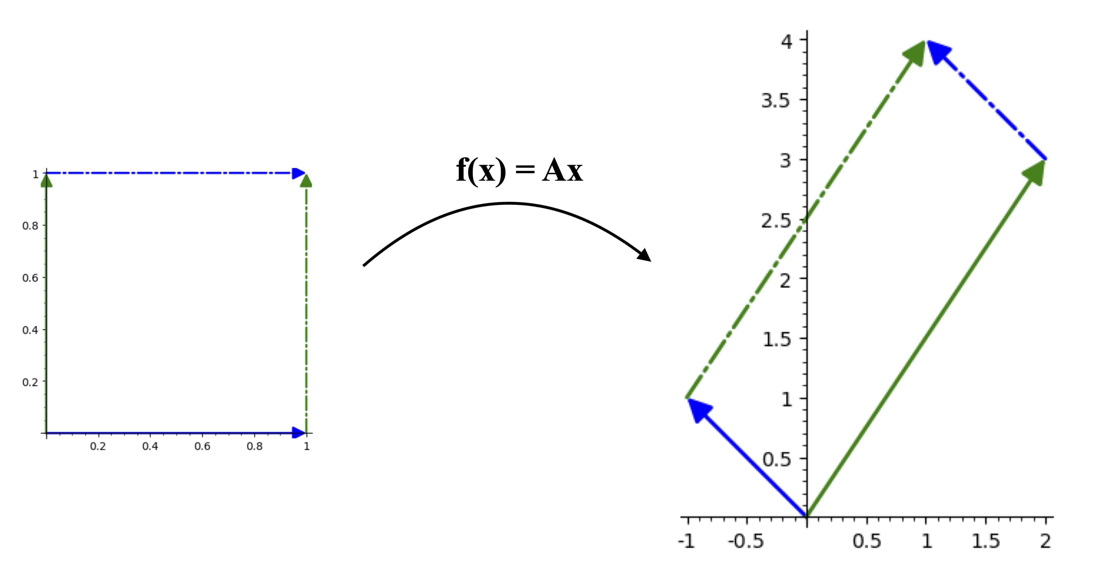
We will consider a small (2 by 2) example matrix to illustrate some of the properties of determinants.

The determinant is $(-1)(3) - (2)(1) = -5$. This means that when this matrix acts on the plane $(x_1,x_2)$, it magnifies areas by a factor of 5 as well as a reflection. Note that the figures below have different scales for the domain and the image planes.

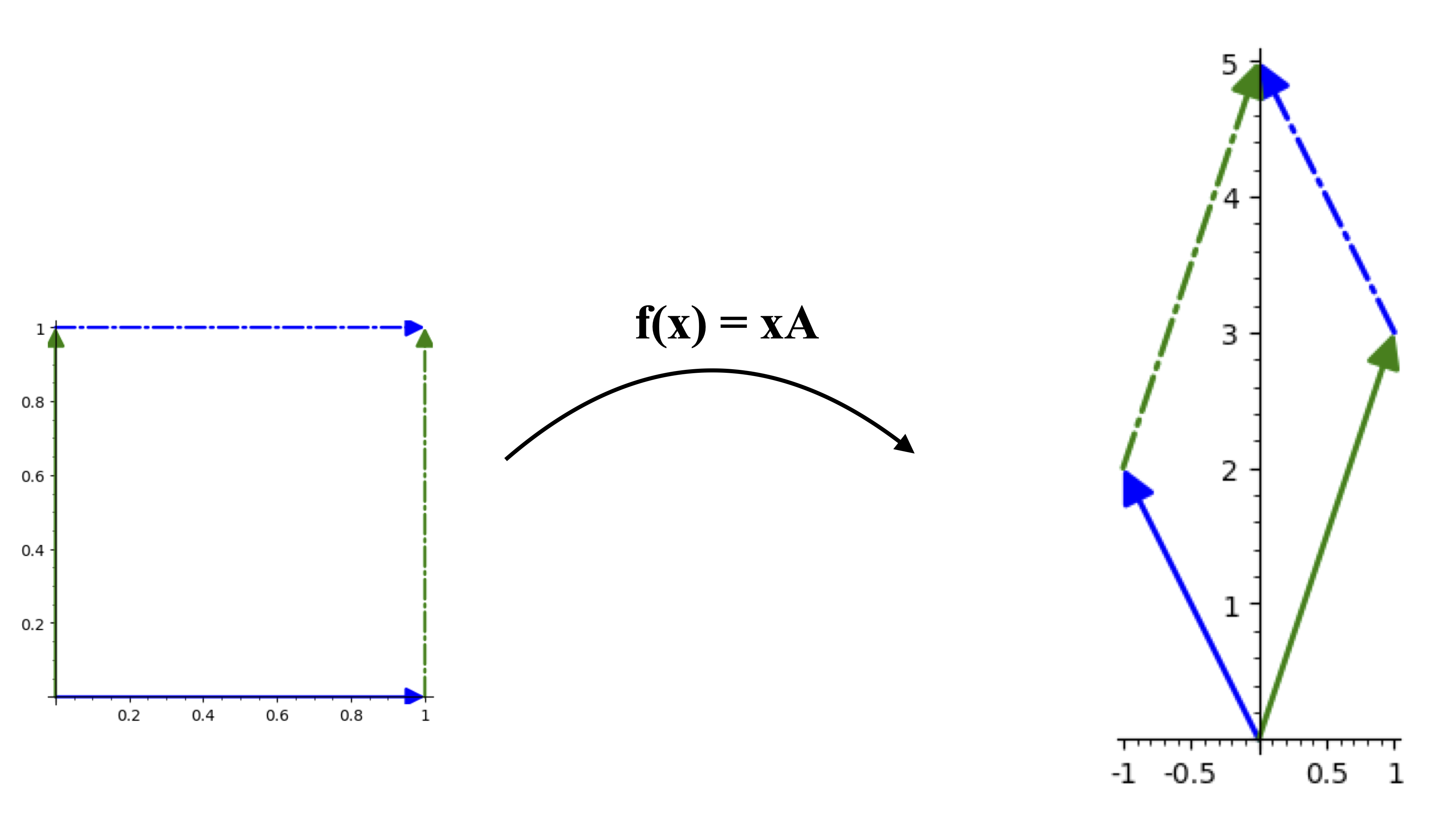
If we consider the matrix as acting from the right, so $f(x) = xA$, then we can see the invariance of the determinant under the transpose operation means the image area is again changed by a factor of -5, even though the mapping is not the same.

---

The Laplace Expansion

For larger $n$ the determinant can be defined recursively through the Laplace expansion formula. If we pick a particular row $i$, then

where $M_{i,j}$ is the determinant of the submatrix of $A$ which is obtaining by deleting row $i$ and column $j$.

The same formula can be used with a fixed column instead of a fixed row,

because $\det(A) = \det(A^T)$.

The sign pattern of the minors in the Laplace expansion is given by $(-1)^{(i+j)}$ for the minor formed by deleting the $i$th row and $j$th column. This is a checkerboard of signs; for example the 4 by 4 pattern is:

---

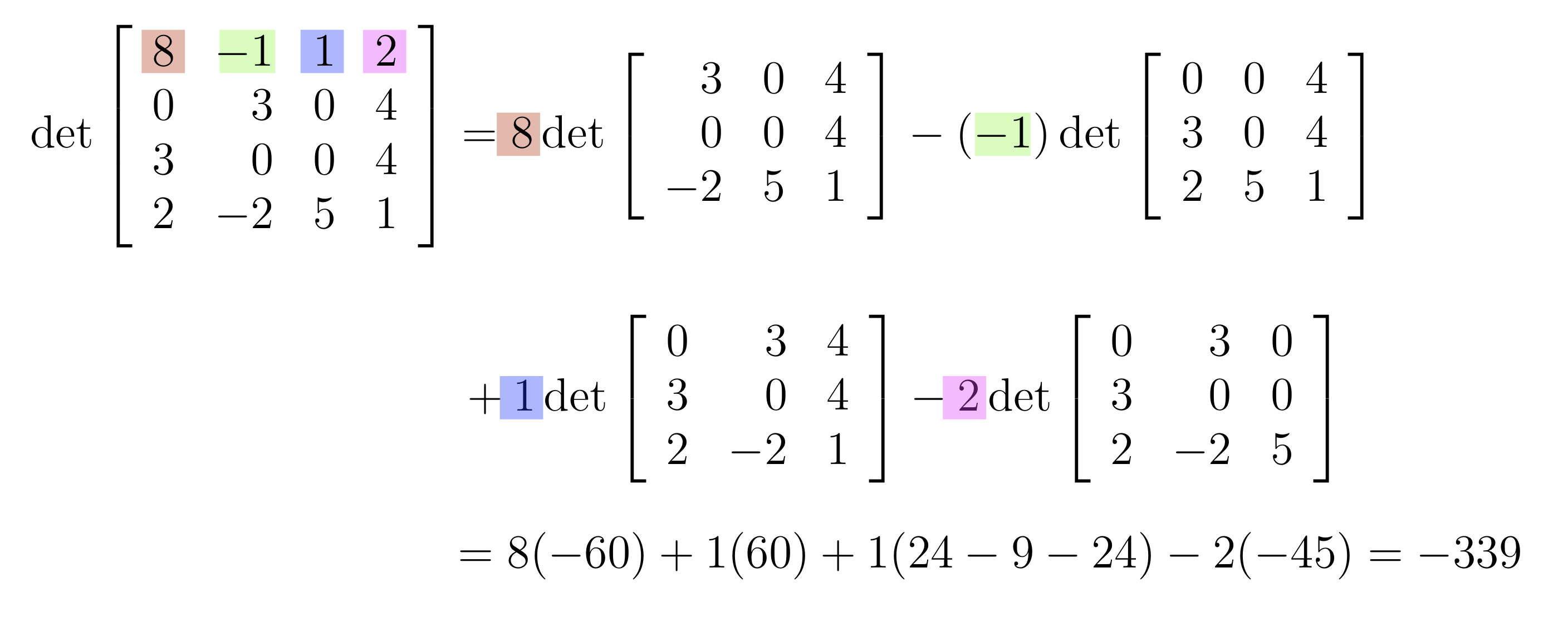
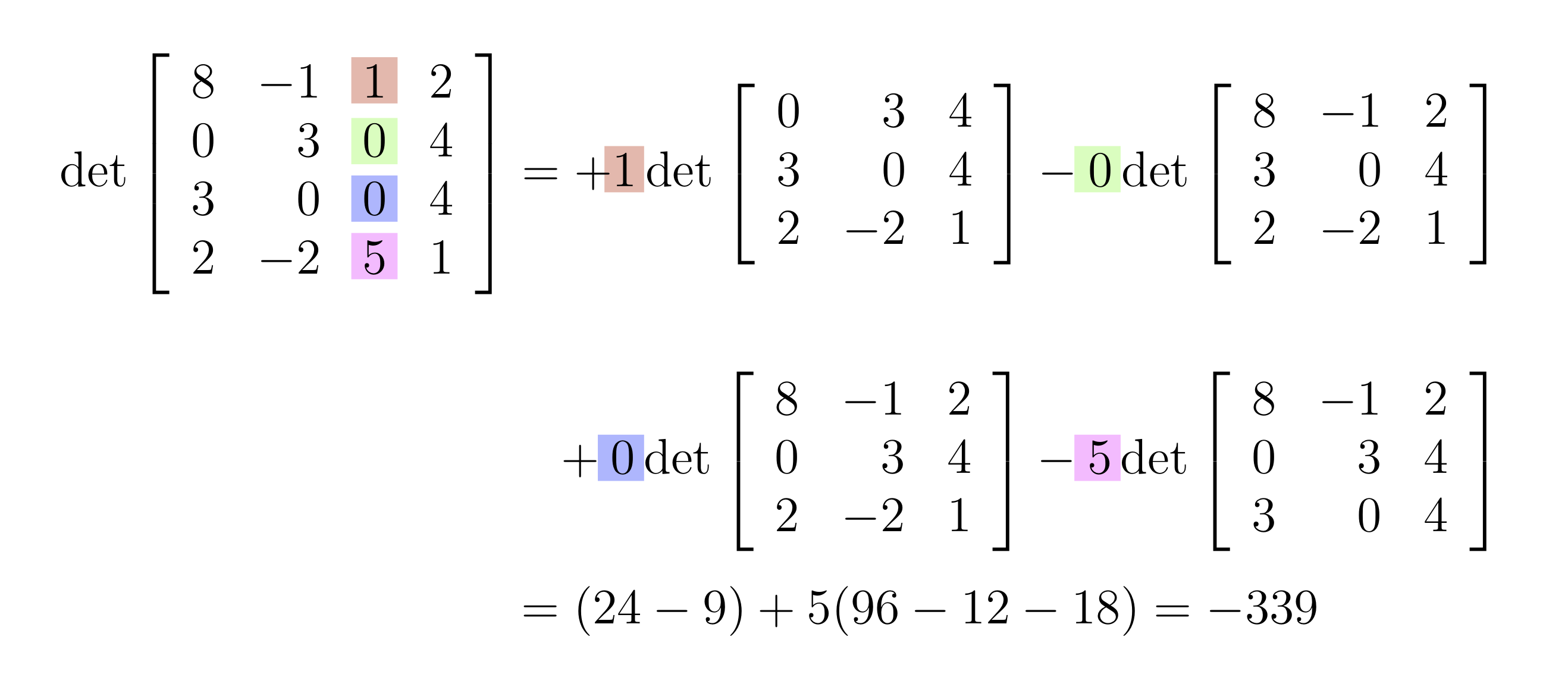
Example: Column vs. row expansion for determinants

Here is an example of comparing using a column instead of a row in the Laplace expansion to compute a 4 by 4 determinant.

---

Efficient determinant computation

The computational cost of directly using the Laplace expansion becomes ridiculous even for moderately large matrices - for an $n$ by $n$ matrix it takes more than $n!$ multiplication and addition operations, so a 30 by 30 matrix determinant would require over $10^{32}$ operations. A single fast computer core capable of $10^{10}$ operations per second would take over 800 trillion years to finish the job. So we need a better way. Fortunately determinants have many interesting properties that we can use to speed up their computation.

The first useful thing we can use is that the determinant of an upper- or lower-triangular matrix is equal to the product of its entries. This is not difficult to prove from the Laplace expansion.

---

Example: Upper-triangular determinant

---

The second useful technique we can use is row and column operations. Some of these change the determinant, so we must keep track of how the answer we want is affected by them. Swapping 2 rows changes the sign of the determinant, and rescaling a row multiplies the determinant by the scaling factor. However, the most useful row operation is adding a multiple of one row to another, which fortunately does not affect the determinant(!). Here are some examples:

---

Examples: row operations and determinants

Swapping rows:

Rescaling rows:

Adding a multiple of one row to another:

---

The same facts hold for column operations, giving us many options to simplify a matrix to upper- or lower-triangular form.

Permutation formula for the determinant

There is another formula for the determinant that is quite different from the recursive Laplace expansion. This is an explicit formula showing that the determinant is a sum over the $n!$ ways of choosing $n$ elements from the matrix from distinct rows and columns; each term is a signed product of these elements:

In this formula we are writing $S_n$ as a shorthand for all of the possible permutations of $n$ elements $\{1, 2, \ldots, n\}$. The sign (either +1 or -1) of each of these permutations $\sigma$ is defined as $(-1)^t$ where $t$ is the number of transpositions (swaps between two elements) needed to convert the identity permutation $(1, 2, \ldots, n)$ to $\sigma$.

If you haven't seen permutations before this is probably very confusing. Lets look at the particular case $n=3$ to illustrate the pieces of the permutation formula.

For $n=3$ there are six permutations: $(1,2,3)$, $(1,3,2)$, $(2,1,3)$, $(2,3,1)$, $(3,2,1)$, and $(3,1,2)$. With this choice of ordering, the determinant formula above for a $3$ by $3$ matrix $A$ is the sum

What are signs of these permutations (the $sgn(\sigma)$)? The first one, $(1,2,3)$, is the identity permutation (it sends 1 to 1, 2 to 2, and 3 to 3), so its sign is $sgn(\sigma) = (-1)^0 = 1$.

The second permutation, $(1,3,2)$, is one transposition away from the identity (swap the 2 and the 3), so its sign is $(-1)^1=-1$.

The third permutation, $(2,1,3)$, is also one transposition away from the identity (swap the 2 and the 1), so its sign is $(-1)^1=-1$.

The fourth permutation, $(2,3,1)$, is two transpositions away from the identity so its sign is $(-1)^2=1$.

The fifth permutation, $(3,2,1)$, is one transposition away from the identity so its sign is $(-1)^1=-1$.

The sixth permutation, $(3,1,2)$, is two transpositions away from the identity so its sign is $(-1)^2=1$.

So the final explicit formula is

The permutation formula is not very useful for directly computing large determinants, but it is important because it shows some of the properties of determinants more clearly than the Laplace expansion.

Eccentric Determinant Computation

A quirky, and somewhat unreliable method of computing determinants was invented by Charles Dodgson (better known through his pen name Lewis Carroll as the author of Alice in Wonderland), called Dodgson Condensation.

---

Exercises:

1. Find a three by three matrix with strictly positive entries ($a_{ij} > 0$ for each entry $a_{ij}$) whose determinant is equal to $1$. A bonus will be given for finding such a matrix with the smallest sum of entries, that is, such that $\sum_{i=1, j=1}^{i=3,j=3}a_{ij} = a_{11} + a_{12} + \ldots + a_{33}$ is as low as possible.

2. The $n \times n$ Vandermonde determinant is defined as:

   $$V(x_1, x_2, \ldots, x_n) = \text{det} \left( \begin{array}{ccccc} 1 & x_1 & x_1^2 & \cdots & x_1^{n-1} \\ 1 & x_2 & x_2^2 & \cdots & x_2^{n-1} \\ \vdots & \vdots & \vdots & \ddots & \vdots \\ 1 & x_n & x_n^2 & \cdots & x_n^{n-1} \end{array} \right )$$

   Show that the $2 \times 2$ Vandermonde determinant $V(a,b) = b - a$. Then show using row operations that the $3 \times 3$ Vandermonde determinant $V(a,b,c)$ can be factored into $(a-c)(b-c)(b-a)$.

3. Compute the determinant of

   $$A = \left[ \begin{array}{rrrr} 8 & -4 & -6 & 4 \\ 2 & 6 & 0 & 4 \\ 6 & 0 & -2 & 4 \\ 4 & -2 & -2 & a \end{array}\right]$$

   using properties of determinants to simplify the calculation (show your steps).

---

Curve-fitting

Linear algebra has many applications outside of differential equations. In this section we will highlight just one of these: interpolation or curve-fitting.

---

Example: Parabolic fit

Suppose we want to find a parabola of the form $y = a_0 + a_1 x + a_2 x^2$ which passes through the points $(1,1), (2,3), (3,7)$. For each $(x,y)$ point we can substitute in the $x$ and $y$ value into the parabola's equation, giving us three linear equations in the unknown parameters $a_0$, $a_1$, and $a_2$:

The coefficient matrix on the left has a special form which arises in this kind of problem; it is called a Vandermonde matrix after the 18th-century musician and mathematician A.-T. Vandermonde.

For this particular trio of points we get the system:

which we can row reduce to

so $a_0 = 1$, $a_1 = -1$, and $a_2 = 1$; the parabola is $y = 1 + x + x^2$.

---

Exercises:

1. Using the equation

find a circle passing through the points $(1,7)$, $(-1,3)$, and $(0,0)$. After finding $A$, $B$, and $C$, put the circle's equation in the standard form

(by completing the squares).

1. Find the ellipse of minimal area which is of the form

and which passes through the points $(x,y) = (1,1)$ and $(x,y) = (-1,2)$.

The area of these ellipses is most easily expressed by writing the equation as

where $M = \left ( \begin{array}{cc} A & B \\ B & C \end{array} \right )$. Then the area of such an ellipse is $\displaystyle \frac{\pi}{\sqrt{\det (M)}}$ (note that the minimal area will occur when $\det(M)$ is maximized).

Least-squares fitting

In the previous section we saw how linearly parameterized curves with $n$ parameters can be fit to $n$ points. This can be very useful in design problems, but it is not as useful in data analysis where we usually want to fit a relatively simple model to data that contains noise and other non-modeled components. That is, for data analysis we want to find a best-fitting curve that has fewer parameters than the number of data points.

The most common choice of "best fit" is to minimize the sum of squared deviations from the curve. This is called "least squares" fitting, and it is very convenient because the derivative of the error is linear and we can use well developed linear algebra methods to efficiently calculate the best fit.

A full discussion of least-squares fitting is beyond the scope of this text, but because of its importance we will briefly summarize how it works in a simple setting.

Suppose we have $n$ data points $(x_i, y_i)$ (with $i \in (1,2,\ldots,n)$) and a model curve

where the number of parameters $a_i$ is $m$, and $m < n$. Evaluating the model at the data points gives us individual equations

which we can write as a matrix equation

in which $Y$ is a $n \times 1$ column vector $(y_1, \ldots, y_n)^T$, $F(X)$ is a $n \times m$ matrix whose ($i$,$j$)th entry is $f_j(x_i)$, and $A$ is a $m \times 1$ column vector of coefficients $(a_1, \ldots, a_m)^T$.

We want to solve the equation for the coefficients in $A$, but this is usually impossible since the $F(X)$ matrix is not square, and thus not invertible. However we can make a new square system that is the projection of the problem onto a solvable problem:

The matrix $G = F(X)^T F(X)$ is now $m \times m$, and can usually be inverted. Our least-squares solution for the coefficients is

For large problems this simple method can have some loss of precision, and more sophisticated methods are preferred (e.g. the "QR" method).

Lets look at a small example to illustrate the method.

---

Example: Least squares fitting

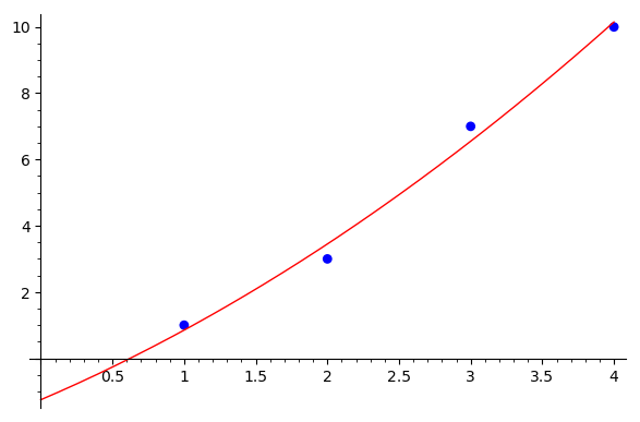
We will extend the curve-fitting example with an extra data point: suppose we want the least-squares fit of a parabola $y = a_0 + a_1 x + a_2 x^2$ for the points $(1,1)$, $(2,3)$, $(3,7)$, and $(4,10)$. The (unsolvable) matrix formulation $Y=F(X)A$ is

We multiply both sides of the equation by $F(X)^T$; on the right this gives us the square coefficient matrix

which has the inverse

and now we can find

So the parabolic fit is

The data and the parabolic fit are shown below. Note that the parabola does not go exactly through any of the data points, which is typical for a least-squares fit.

---

Matrix transformations in computer graphics

Although the first use of matrices was for solving systems of linear equations, they are used for many purposes beyond that. Perhaps the most common use of all for matrices is representing linear transformations in 2 and 3 dimensions for computer graphics. We will briefly describe the 3-dimensional case, which can be easily truncated to obtain the 2-dimensional version.

The linear operations we want to represent are rigid motions and rescalings of objects: rotations, translations, and scaling. These can all be incorporated into one more general transformation matrix if we use projective coordinates for the object. Instead of using $(x,y,z)$ we add an additional coordinate to get $(x,y,z,1)$. This may look odd at first but it ends up unifying and simplifying our transformations.

To help see the point of using projective coordinates let's look first at translations. A translation of a 3-D vector $v = (x,y,z)^T$ by a displacement vector $a = (a_1, a_2, a_3)^T$ can be written as:

With projective coordinates we can write this as a matrix multiplication instead. If $w = (x,y,z,1)^T$, then

In the projective framework if we rescale the $x$, $y$, and $z$ directions by scaling factors $S_x$, $S_y$, and $S_z$ we use the matrix

Rotations are more complex (pun intended). One way to think of them in matrix terms is to compose a series of rotations around different axes. For example, to rotate around the x-axis by $\theta$ radians we can use the matrix:

Exercise:

1. Using projective coordinates $v = (x,y,1)^T$, construct 3x3 transformations matrices $T_1$ and $T_2$ such that $T_2 \circ T_1$ rotates by an angle $\pi/4$ around the point $(1,1)$ (i.e. $(1,1,1)^T$ in projective coordinates).

Additional Exercises

1. A linear system of the form:

   $$a_{11} x + a_{12} y = 0$$
   $$a_{21} x + a_{22} y = 0$$

   is said to be homogeneous (i.e. when the right hand side is zero). Explain in geometric terms why such a system must either have a unique solution or infinitely many solutions. Compute the unique solution when it exists.

2. Use elementary row operations to transform the augmented coefficient matrix of the system below into echelon or reduced echelon form. Use this to write down all the solutions to the system.

   $$\begin{split} x + 2 y + -2z & = 3 \\ 2x +4 y - 2 z & = 2 \\ x + 3 y +2 z & =-1 \end{split}$$

3. Same as above, for the system:

   $$\begin{split} x + 2 y - z & = -1 \\ x + 3 y - 2 z & = 0 \\ -x - z & = 3 \end{split}$$

4. Under what conditions on the numbers $a$, $b$, and $c$ does the following system have a unique solution, infinitely many solutions, or no solutions? $$ \begin{split} 2x - y + 3z & = a \ x + 2 y + z & = b \ 6x + 2y + 8z & = c \end{split} $$

5. Reduce the following matrix to reduced row echelon form.

   $$\left ( \begin{array}{rrr} 1 & 3 & -6 \\ 2 & 6 & 7 \\ 3 & 9 & 1 \end{array} \right )$$

   13-15. For the following three pairs of matrices, compute whatever products between them are defined.

6. $$A = \left ( \begin{array}{rrr} 1 & -2 & 1 \end{array} \right ), B = \left ( \begin{array}{rrr} 1 & 3 & 0 \\ 1 & 2 & 1 \end{array} \right )$$
7. $$A = \left ( \begin{array}{rrrr} 2 & 0 & 1 & 0 \end{array} \right ), B = \left ( \begin{array}{rr} 1 & 0 \\ 0 & 2 \end{array} \right )$$
8. $$A = \left ( \begin{array}{r} 3 \\ 4 \end{array} \right ), B = \left ( \begin{array}{rr} 1 & 1 \\ 2 & 2 \\ -1 & 1 \end{array} \right )$$

9. Find a two by two matrix $A$ with all non-zero entries such that $A^2 = 0$.

10. Find a two by two matrix $A$ with each diagonal element equal to zero such that $A^2 = -I$. (The existence of such matrices is important, as it lets us represent complex numbers by real matrices).

11. Find the inverse $A^{-1}$ of the following matrix by augmenting with the identity and computing the reduced echelon form.

    $$A = \left(\begin{array}{rrr} 5 & 3 & 6 \\ 4 & 2 & 3 \\ 3 & 2 & 5 \end{array}\right)$$

12. Compute the inverse of $A$ to find a matrix $X$ such that $AX=B$ if

    $$A = \left(\begin{array}{rr} 5 & 3 \\ 3 & 1 \end{array}\right)$$

    and

    $$B = \left(\begin{array}{rrr} 3 & 2 & 4 \\ 1 & 6 & -4 \end{array}\right)$$

13. Show that if $A$, $B$, and $C$ are invertible matrices then $(ABC)^{-1} = C^{-1}B^{-1}A^{-1}$.

14. Compute the determinant of

    $$A = \left(\begin{array}{rrrr} 3 & 1 & 0 & 2 \\ 0 & 1 & 20 & 2 \\ 0 & 0 & 1 & -63 \\ 9 & 3 & 0 & 1 \end{array}\right)$$

15. Show that if a matrix $A$ has the property $A^2 = A$, then either $\det(A) = 0$ or $\det(A) = 1$.

16. Find a quadratic polynomial $a_2 x^2 + a_1 x + a_0$ whose graph passes through the points $(1,3)$, $(2,3)$, and $(4,9)$.

17. Determine whether the vectors $(0,2)$ and $(0,5)$ are linearly dependent or independent.

18. Express $w = (1,2)$ as a linear combination of $u = (-1,-1)$ and $v = (2,1)$.

19. Calculate the determinate of the matrix whose columns are $u$, $v$, and $w$ to determine if $u$, $v$, and $w$ are linearly independent or not, with $u = (-2, -5, -4)^T$, $v = (5,4,-6)^T$, and $w= (8,3,-4)^T$.

Review

1. Compute the value of $y(1)$ if $y' = 2 x y^2$ and $y(0) = 2$.

2. Approximate $y(1)$ from the previous problem using Euler's method with 2 steps. Compare that approximation to that given by the improved Euler method with 1 steps, and the Runge-Kutta method using 1 step. Which is the best approximation?

3. Solve the initial value problem $\displaystyle \frac{d y}{d x} = 3 \frac{y}{x} - 3\ x^5$, $\ y(2) = 56$.

4. Compute the inverse of the matrix

   $$A = \left(\begin{array}{rrr} b & b & 0 \\ b & b & b \\ 0 & b & b \end{array}\right)$$

   where $b \neq 0$.

5. Draw a phase diagram covering the interval $(-8,8)$ for the differential equation $\displaystyle \frac{dy}{dt} = y \sin^2(y)$, including the equilibria, the direction of solutions, and the stability of the equilibria. In addition, sketch the solutions $y(t)$ for representative initial $y$ values in the interval $(-8,8)$.

6. Characterize the $2$ by $2$ matrices $A$ which have the property that $\det(A + A) = \det(A) + \det(A)$.

7. Compute the inverse of

   $$A = \left[ \begin{array}{rrr} \cos(\theta) & -\sin(\theta) & 0 \\ \sin(\theta) & \cos(\theta) & 0 \\ 0 & 0 & -1 \\ \end{array}\right]$$

Notes

Notes: (Local storage in a cookie) Add

License

This work (text, mathematical images, and javascript applets) is licensed under a Creative Commons Attribution-NonCommercial-ShareAlike 4.0 International License. Biographical images are from Wikipedia and have their own (similar) licenses.