Part 1: Sequence Alignment, Evolution, Entropy, and Information
Sequence alignment algorithms
The alignment of two or more sequences (primarily DNA, RNA, or protein) is perhaps the most fundamental problem in bioinformatics. Its importance is reflected in the vast literature on the subject. In this chapter we will survey some of the most basic and core ideas in the theory of alignments.
Below is an example of an alignment of two DNA sequences. The top sequence is from a portion of the human gene alpha-actin, which is one of the components of muscle fibers that enables muscles to contract. The bottom sequence is from the chicken (Gallus gallus). Identical bases are indicated with lines connecting them, and a gap in one sequence relative to another is shown with a dash.
ATGTGTGAAGAAGAGGACAGCACTGCCTTGGTGTGTGACAATGGCTCTGGGCTCT-GT-A
|||||||| || || || | ||| ||  | ||||| ||||| |||||  ||| || || |
ATGTGTGACGAGGACGAGACCACCGCGCTCGTGTGCGACAACGGCTC-CGGC-CTGGTGA
Number of alignments
The number of possible alignments between two sequences is so huge, even for moderate length sequences, that we must be very efficient in search for an optimal alignment. Two sequences of length n have approximately 2^{2n} n^{-1/2} alignments; for n=20 this is about 1.38 \times 10^{11}. When sequencing DNA it is common to want to align a sequenced read, typically of length 50 to 250, to a database with millions or possibly billions of letters (bases). Even worse, we often want to compare multiple sequences together, and then the problem really gets computationally intractable for exact results.
Needleman-Wunsch global pairwise alignment
Starting in the late 1960s the problem of efficient sequence alignment began to be studied intensively. The first algorithm we will consider is the dynamic programming (see below) algorithm of Needleman and Wunsch. It is a global pairwise alignment algorithm, which means that all of the letters in each of two given sequences will be part of the alignment.
It is assumed that we have a scoring matrix for the alignment, which rewards matching identical (or similar) letters and penalizes mismatches. The total score of an alignment is the sum of each of the scores of each pair in the alignment. We must also have a penalty for gaps - alignments of letters from one sequence with nothing from the other. We will discuss gap penalties in more detail later; for now we will just use a linear gap penalty that lowers the score by a constant amount g for every gap.
The main idea of the algorithm is to keep track of the best scoring alignment that uses i letters from the first sequence and j letters from the second sequence. We store the scores of these alignments in a table B(i,j). The table is initialized by the convention that the empty alignment of no letters has a score of 0, i.e. B(0,0) = 0. Two of the borders of the table consist of alignments with letters from only one of the sequences, which consist of gaps, so B(i,0) = -g i and B(0,j) = -g j.
The efficiency of the algorithm comes from the fact that we can recursively determine B(i,j) from previous entries rather than optimizing the entire alignment from scratch. The best scoring alignment using i and j letters can be formed from a previous alignment by adding a letter from each sequence, or just one letter aligned with a gap. We choose the highest scoring of these three choices. This gives the formula:
where the first sequence is a_1 a_2 \ldots a_n and the second is b_1 b_2 \ldots b_m. Besides determining B(i,j) for each i and j, we must keep track of the choice we made at each step if we want to reconstruct the alignment itself.
It is easiest to describe the algorithm with a concrete example. We will use a simple scoring matrix S that awards one point for each exact match, and subtracts a point for any mismatched letters. The linear gap penalty constant g will be -2. The matrix S is shown below:
| A | C | G | T | |
|---|---|---|---|---|
| A | 1 | -1 | -1 | -1 |
| C | -1 | 1 | -1 | -1 |
| G | -1 | -1 | 1 | -1 |
| T | -1 | -1 | -1 | 1 |
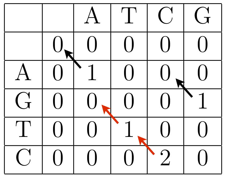
We will align the two sequences ATCGG and AGTCG. The initialized score table is:
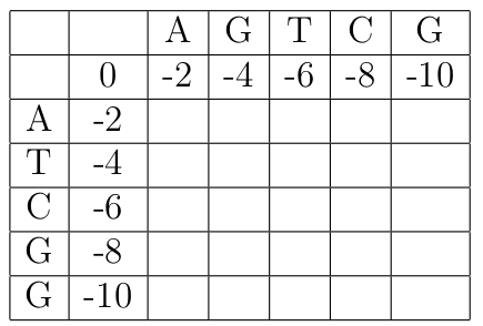
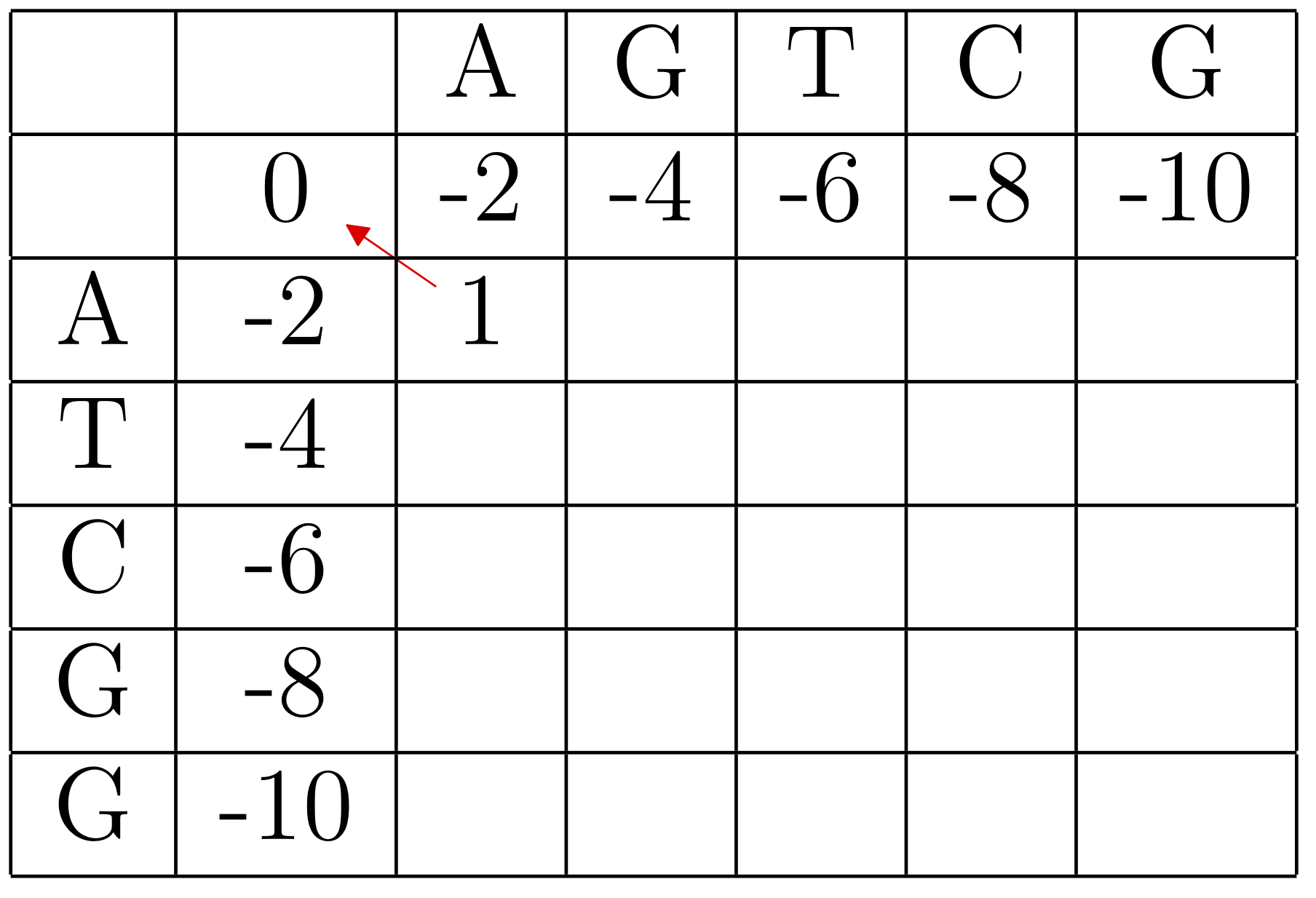
The first entry we compute is B(1,1). In this case, since a_1 = b_1 = A, the maximum score is obtained by a match, giving a score of B(0,0) + S(A,A) = 0 + 1 = 1. We can graphically keep track of this choice with a diagonal arrow.
The completed table, along with arrows indicating the backtracking:
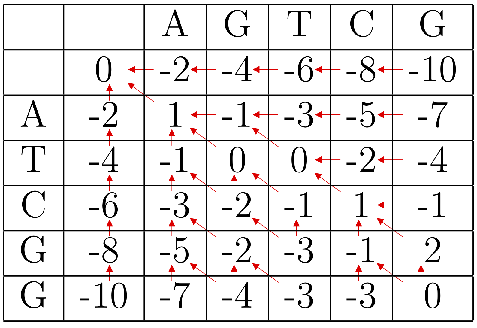
We can recover the best alignments by tracing back from the lower right entry, which is the overall score of the alignment. In this case there was a tie, so there are two possible paths, corresponding to the two alignments:
                                 A-TCGG
                                 AGTC-G


                                 A-TCGG
                                 AGTCG-
Smith-Waterman local pairwise alignment
Often we do not want a global alignment, but rather to find a good match of substrings of the two sequences. This is a local alignment. The Needleman-Wunsch algorithm can be modified a little to accomplish this, which is the Smith-Waterman algorithm. The changes we need to make are to consider a matrix of values L(i,j) = max(0,B(i,j)), where B(i,j) is given recursively as before, and to trace back from the maximum entry in the matrix (instead of the lower right corner). So the recursive scoring becomes
The purines, A (adenine) and G (guanine) are complementary to the pyrimidines C (cytosine) and T (thymine); it is more common for purines to mutate to purines, and pyrimidines to pyrimidines (transitions), than for one type to change to the other (a transversion). So one might penalize a transition mismatch less, such as the scoring matrix:
| A | C | G | T | |
|---|---|---|---|---|
| A | 2 | -2 | -1 | -2 |
| C | -2 | 2 | -2 | -1 |
| G | -1 | -2 | 2 | -2 |
| T | -2 | -1 | -2 | 2 |
Example: Using the scoring matrix above with a linear gap penalty of -3 per indel, we begin by bordering the dynamic programming matrix with zeros.
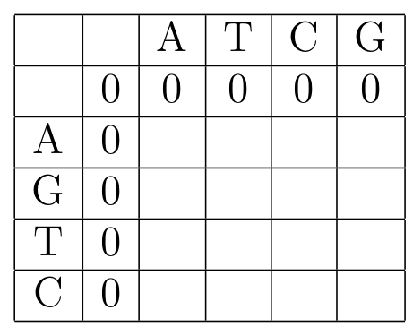
Then we proceed as before, but it is only worthwhile to keep track of the optimal direction for cells with positive entries.
The local optimal alignment is
    TC
    TC
Exercise:
Exercise 1: Change the Needleman-Wunsch implementation below to the Smith-Waterman algorithm (i.e. from global to local alignment).
-
change the score in each cell so that it is at least 0
-
change the initial scores along the edge of the table to 0
-
start the traceback from the maximum score (instead of the bottom corner)
-
end at a cell with a positive score
    # load a standard protein scoring matrix
    from Bio.Align import substitution_matrices
    b62 = substitution_matrices.load("BLOSUM62")

    #Needleman-Wunsch function:
    def NW(string1, string2, scoring_dict = b62, gap = -6, verbose = True):
        """
        Performs Needleman-Wunsch alignment of string1 and string2.
        Returns the array of scores and pointers(arrows).
        If verbose=True (the default) then the alignment is printed
        out as well.

        EXAMPLE:
            Scores, Pointers = NW('Pelican', 'trellisant', verbose = True)
            P-E-LICAN-
            TRELLISANT
            Score: 3
        """
        # Initialize scoring and 'arrow' (traceback) matrices to 0
        Scores = [[0 for x in range(len(string2)+1)] \
            for y in range(len(string1)+1)]
        Pointers = [[0 for x in range(len(string2)+1)] \
            for y in range(len(string1)+1)]

        # Convert to uppercase:
        string1 = string1.upper()
        string2 = string2.upper()

        # Initialize borders.
        # For pointers (arrows), use 2 for diagonal, -1 for horizontal,
        # and 1 for vertical moves (these are completely arbitrary codes).
        # The index i is used for rows (vertical positions) in the score
        # and pointer tables, and j for columns (horizontal positions).
        for i in range(len(string1)+1):
            Scores[i][0] = gap*i
            Pointers[i][0] = 1
        for j in range(len(string2)+1):
            Scores[0][j] = gap*j
            Pointers[0][j] = -1

        # Fill the dynamic programming table with scores
        for i in range(1,len(string1)+1):
            for j in range(1,len(string2)+1):
                letter1 = string1[i-1]
                letter2 = string2[j-1]
                DiagScore = Scores[i-1][j-1] + scoring_dict[(letter1, letter2)]
                HorizScore = Scores[i][j-1] + gap
                UpScore = Scores[i-1][j] + gap
                # TempScores is list of the three scores and their pointers
                TempScores = [[DiagScore,2],[HorizScore,-1],[UpScore,1]]
                # Now we keep the highest score, and the associated direction
                Scores[i][j], Pointers[i][j] = max(TempScores)

        # backtrace from the last entry.
        [i,j] = [len(string1),len(string2)]
        align1 = ''
        align2 = ''
        while [i,j] != [0,0]:
            if Pointers[i][j] == 2:
                align1 = align1 + string1[i-1]
                align2 = align2 + string2[j-1]
                i = i - 1
                j = j - 1
            elif Pointers[i][j] == -1:
                align1 = align1 + '-'
                align2 = align2 + string2[j-1]
                j = j - 1
            else:
                align1 = align1 + string1[i-1]
                align2 = align2 + '-'
                i = i - 1

        # the alignments have been created backwards,
        # so we need to reverse them:
        align1 = align1[::-1]
        align2 = align2[::-1]

        # print out alignment if desired (if verbose==True)
        if verbose == True:
            print(align1)
            print(align2)
            print('Score: ' + str(Scores[len(string1)][len(string2)]))

        # in case you want to look at the scores and pointers,
        # the function returns them
        return [Scores,Pointers]
Affine and other gap penalty functions
There are many reasons for thinking that once there is a gap in an alignment, it should not cost as much to extend the gap. As one example, consider the following part of a multiple alignment of the histone 2B gene:
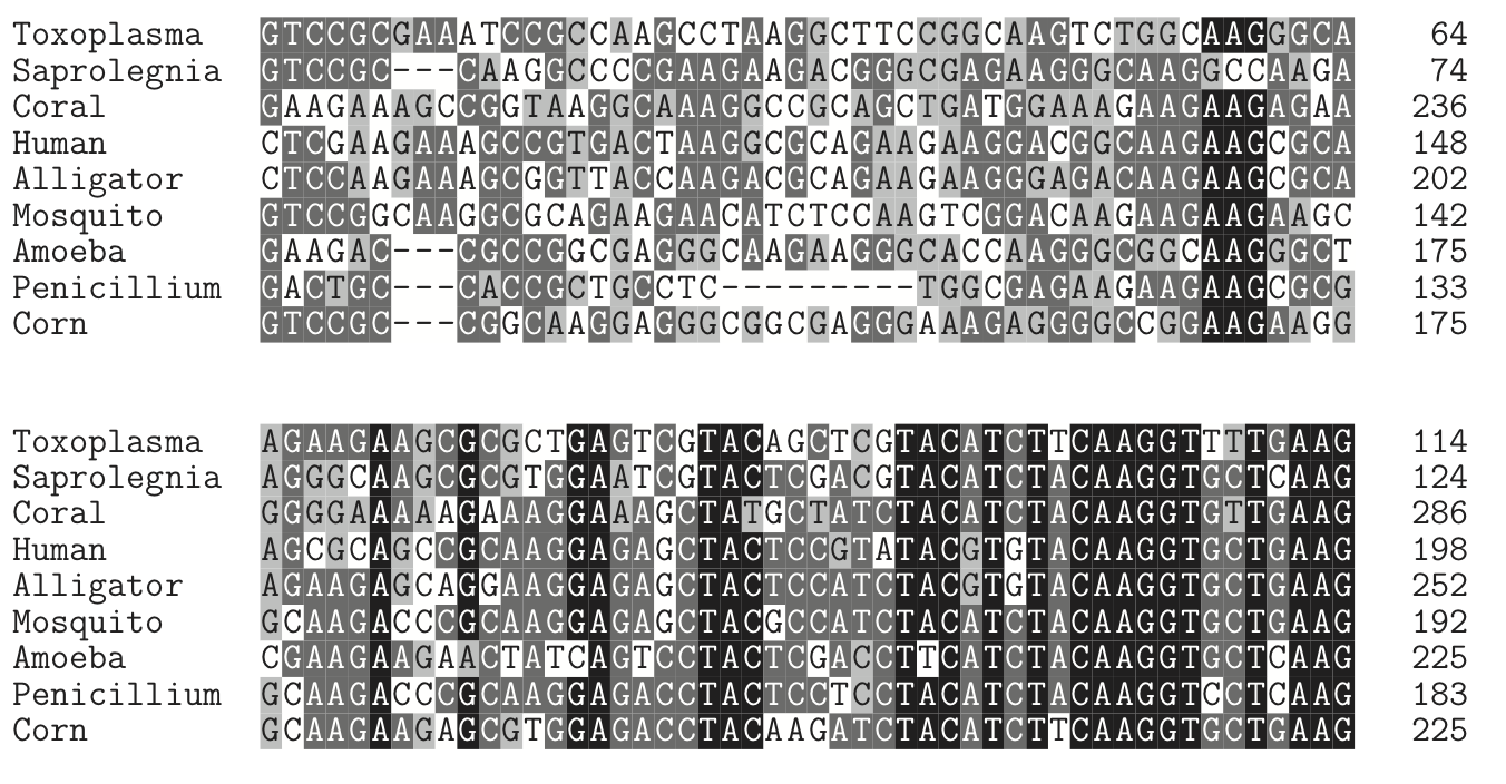
It is clear that in this case the gaps tend to occur in groups - of length 3 and 9 (why are they multiples of three?). To reflect this reality, we would like to use a gap penalty function g(l) with increasing slope. l is the length of a gap. (Often people talk about gap penalties in terms of the 'gap cost' -g(l), in which case we would like a decreasing slope.) But a complicated g(l) will make alignments too computationally expensive; in general we can use the dynamic programming relation:
but for two sequences of length N this now requires O(N^3) operations compared to the O(N^2) for Needleman-Wunsch.
The compromise that has been found is to use an affine gap penalty of the form: $$g(l) = -d - (l-1)e $$ where 0 < e < d. For a specific example, lets consider a scoring system where any match is given 2 points, any mismatch -1, and an affine gap penalty g(l) = -5 -(l-1)1 (so d = 5 and e = 1). With this system, consider the alignments
                1.GGGACAGGG          2.GGGACAGGG
                  GGG-C--GG            GGG---CGG
The gaps in alignment 1 contribute -5 and -6, and the 6 matches give 12, for a total of 1. Alignment two has a score of -7 (the gap) -1 (the mismatch) +10 (5 matches) = 2. The low cost of extension means that having one continuous gap trumps the exchange of a match and mismatch.
Gotoh affine penalty algorithm
The Gotoh algorithm extends the previous algorithms to the affine gap penalty case efficiently by using three tables M, I, and J. The table M keeps track of the best alignment scores using i and j letters which end with a pairing (not a gap); the other two matrices store alignment scores that end with a gap in one of the two respective sequences. This gives the recursion formulae:
The M(i,j) table needs to be initialized with M(0,0) = 0, M(1,0) = M(0,1) = -d, M(0,j) = -je (for j>1) and M(i,0) = -ie (for i > 1) for this form of recursion to work correctly. The I and J table edges should be forbidden (initialized to -infinity or some very large negative number), since it doesn't make sense to do a gap extension from an empty alignment.
Example
For the sequences AATTAAC and AAAAG, if we use the Gotoh algorithm with a scoring of 2 points for a match, -1 points for any mismatch, and an affine gap penalty with -2 points for opening a gap and -1 points for extending a gap, we obtain the I, J, and M tables shown below.
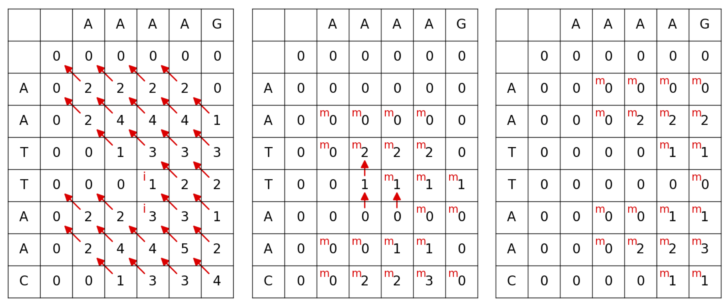
Tracing back from the maximum score of 5 gives the alignment
AATTAA
AA--AA
The Gotoh algorithm was improved to be more efficient by Myers and Miller in 1988 using an idea presented first by Hirschberg, a divide-and-conquer approach that reduces the space (memory) required from O(NM) to O(N) where the two sequences are length N and M and N < M. This efficient version is used as part of many heuristic alignment algorithms such as BLAST.
A note on Dynamic Programming
The Needleman-Wunsch algorithm was described above as a "dynamic programming" algorithm. The Smith-Waterman and Gotoh variants are also dynamic programming algorithms. What does this mean? It is worth spending some time thinking about this, because many of the other algorithms we will discuss in this text use dynamic programming, and its a very useful concept to grasp. In fact we can put forth an only slightly humorous thesis: the first person to think of using dynamic programming in any bioinformatics application gets an algorithm named after them.
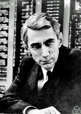
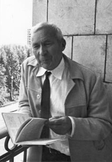
First of all, it may be helpful to know that the term 'dynamic programming' is sort of a joke. It was coined by the brilliant mathematician Richard Bellman, who was working on a government grant through the RAND Corporation in the 1950s. The Secretary of Defense, who oversaw such grants, at that time was known to be a little hostile to mathematics in general, so Bellman tried to choose a name for his work that 'not even a Congressman could object to'. In his autobiography Eye of the Hurricane, Bellman says that "it’s impossible to use the word dynamic in a pejorative sense", and at that time the word 'programming' was used more generally than it is now, to refer to planning and determination of future actions.
Perhaps a better name for dynamic programming would be 'recursive optimization'. It applies to problems with some degree of uniformity in their structure. Sequence alignment is a fairly simple example: aligning two sequences of lengths n_1 and n_2 is structurally very similar to aligning two sequences of lengths n_1-1 and n_2, or of lengths n_1 and n_2 -1, and solving the second problem for substrings of the first problem can be viewed as most of the work in solving the first problem.
Throughout the rest of the text, keep your eye out for this kind of structure.
Fast heuristic alignment and assembly methods
FASTA and BLAST
The dynamic programming algorithms discussed in the previous chapter are insufficiently fast for many applications. In response, many heuristic methods have been developed. Although these methods do not guarantee that an optimal solution is found, they work very well in practice since most of the time we are comparing sequences with a reasonably high degree of similarity.
One of the first heuristic programs was the FASTA family, developed in the late 1980s. Although no longer widely used, its general strategy of first finding high similarity regions using short substrings (k-mers) and then performing local alignments has influenced many current algorithms, including NCBI's BLAST+ suite. The FASTA program also used an input file format which has become the standard for plain-text simple sequence files (see the appendix for more details).
The Burrows-Wheeler Transform and suffix trees
In this section we discuss one of the most fascinating algorithmic tools used in some ultrafast alignment and assembly programs, the Burrows-Wheeler Transform (BWT). The BWT was first developed by David Wheeler in the late 1970s, but did not become widely used until about 20 years later in joint work with Micheal Burrows. The initial application was in compression algorithms, but it has other useful properties for text processing.
It is easiest to understand what the BWT does by seeing an example. The BWT produces a permutation of an input string; for our example we will use the string BANANA. To construct the transform, we augment the string with a special end-of-string symbol, $, cyclically permute the augmented string, and sort the rows lexicographically (we consider the character $ to come after the letter Z):
The BWT is the string in the last column of the sorted output: BNN$AAA. Other treatments of the special end-of-string character will produce slightly different versions of the BWT.
The short story 'the house that Jack built' is a more interesting example which shows some of the power of the BWT:
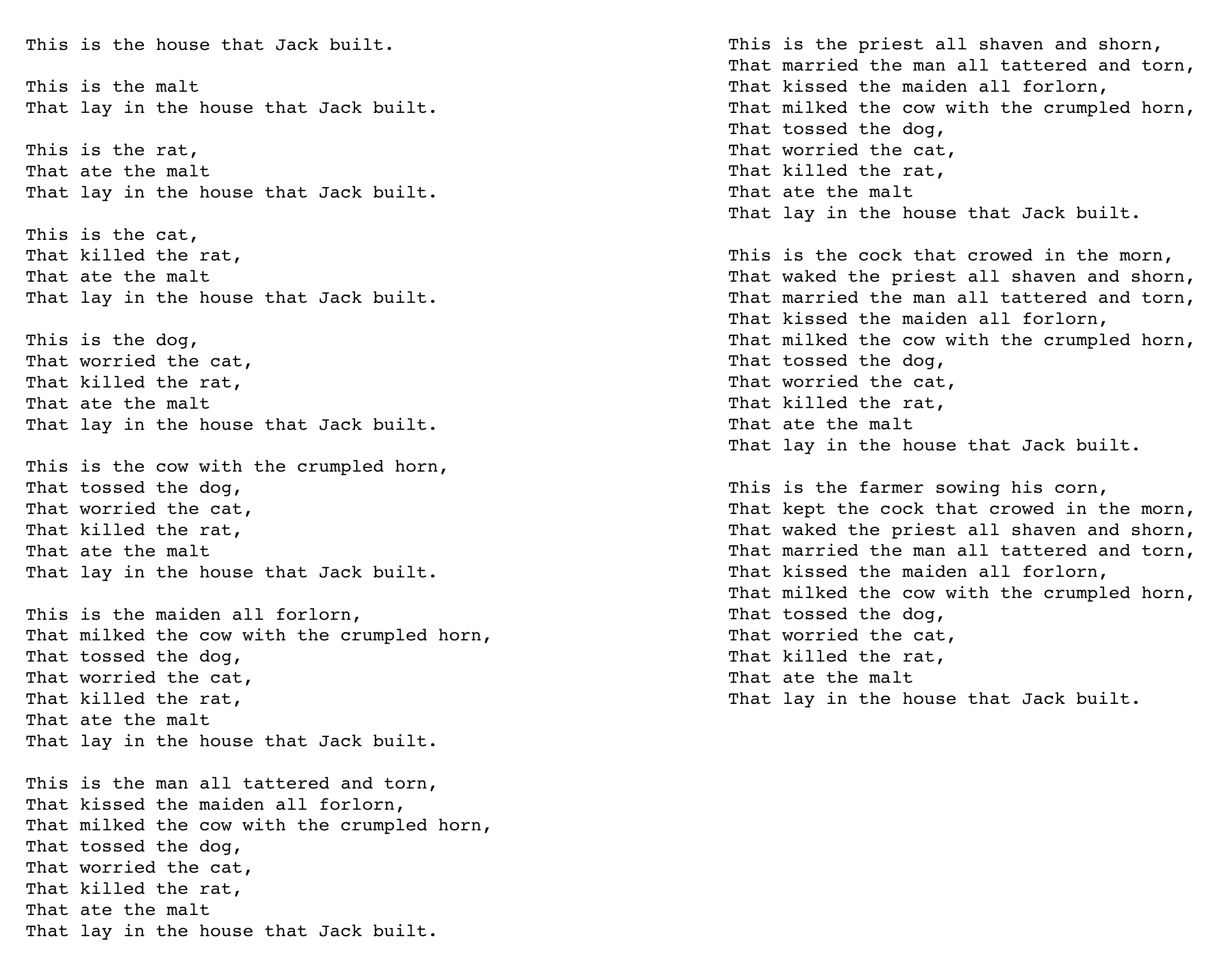
and here is the BWT of that text:
The most striking thing about the transform is how it seems to cluster letters together. This may not seem impressive until you realize that the BWT is an invertible transform - there is no loss of information despite the apparent sorting of the input. To invert the transform, put the output in a matrix as a column, and sort the rows using the same rules used in the original transform. Then add the output in again as the second column, and sort the rows again. Repeat this process of appending the output as a column and sorting until a square matrix is obtained. After sorting the rows of this final matrix, the inverse of the output will be in the last row.
The BWT is closely related to suffix trees. Suffix trees are data structures constructed from strings that are useful for searching within the string. A suffix tree for a string S = a_1a_2\ldots a_n of length n must have the following properties:
-
The tree has exactly n leaves.
-
Except for the root, every internal node has at least two children.
-
Each edge is labeled with a non-empty substring of S.
-
No two edges starting out of a node can have labels beginning with the same character.
-
The string obtained by concatenating all the string-labels found on the path from the root to leaf i spells out suffix a_{n-i}a_{n-i+1}\ldots a_{n}
Below is an example of the suffix tree for the Hawaiian word malamalama (light).
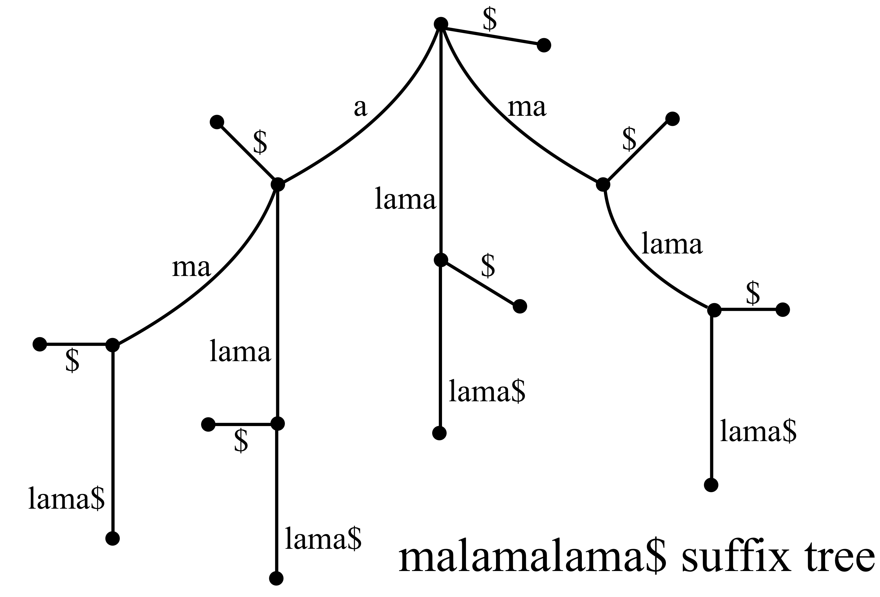
There are efficient algorithms for constructing suffix trees (linear in the size of the text), so if you know you will want to search a given text (such as a genome) many times it is worth creating a suffix tree. The connection of general substring searchs to suffixs arises from the simple fact that every substring is the prefix to a suffix.
Exercise:
-
Compute the Burrows-Wheeler transform of the string HOOHOO\$. The symbol \$ indicates the end of a string, and should be considered to come lexicographically after any other character.
-
Use the work you did in the previous exercise to help construct a suffix tree for HOOHOO\$. (The edges coming out of each node should be labeled with distinct starting letters, and every suffix should be constructable along a path from the root node.)
de Brujn graphs
Another idea that is important in many modern sequence assembly algorithms is that of the de Bruijn graph. In the context of DNA assembly, a k-mer be Bruijn graph consists of vertices v_a = (a_1, a_2, \ldots, a_k), with a directed edge from v_a to v_b if a_i = b_{i-1} for i > 1. In other words the edge indicates that the last k-1 letters of v_a are the first k-1 letters of v_b.
If we consider all k-mers of n symbols, then a cyclic path through the de Bruijn graph of the k-mers that goes through each vertex exactly once (a Hamiltonian path) generates a de Bruijn sequence by concatenating the k-mers along the path. Considered as a cyclic sequence, every k-mer appears once as a substring of the de Bruijn sequence. For example, for the 64 codons (3-mers) of the genetic code, with letters A, C, G, and T, one possible de Bruijn sequence is:
AAACAAGAATACCACGACTAGCAGGAGTATCA
TGATTCCCGCCTCGGCGTCTGCTTGGGTGTTT
The complete de Bruijn graph for the 2-mers of the four DNA letters is shown below:
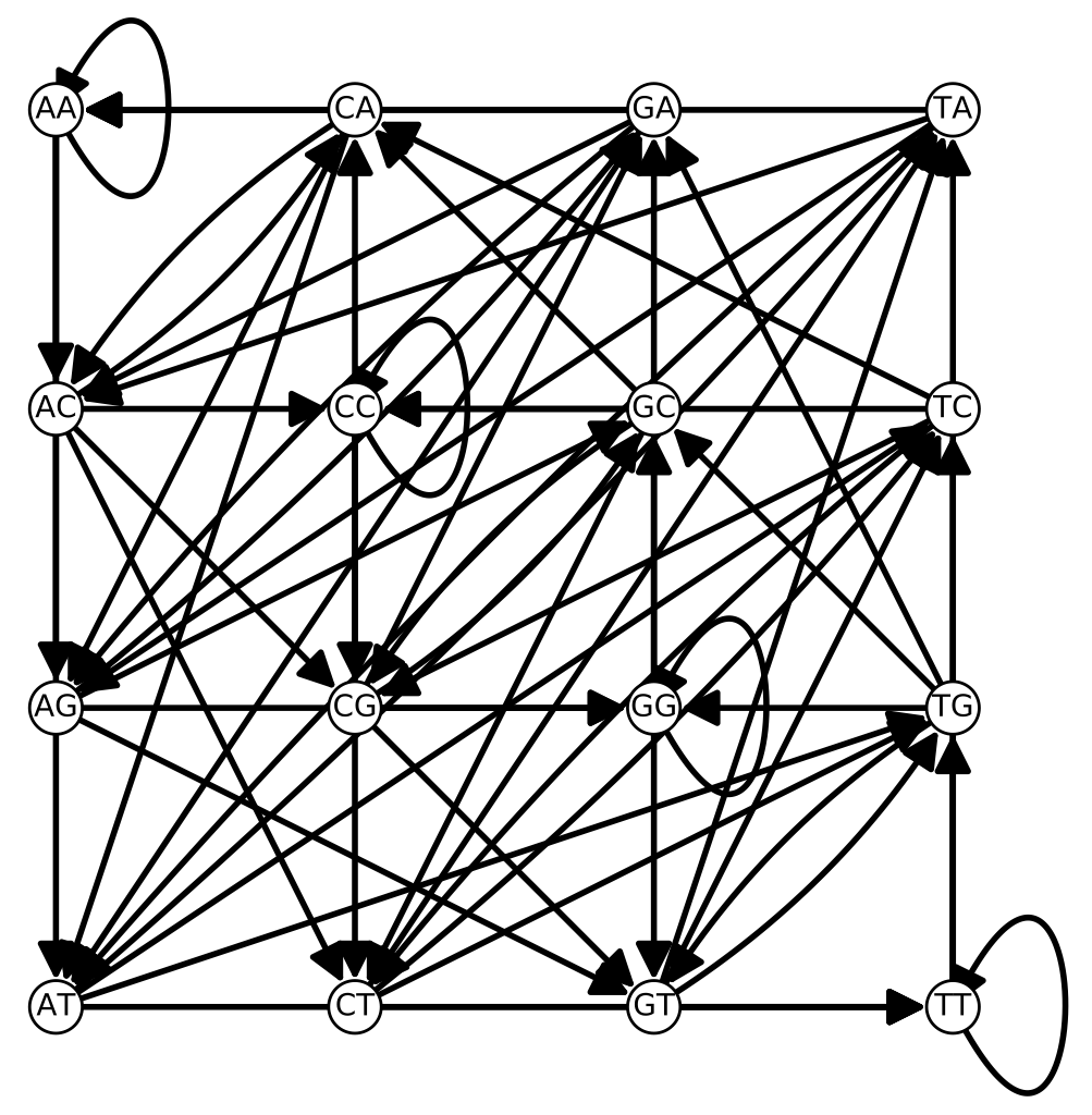
de Bruijn graphs are heavily used in several popular programs such as the fast pseudo-aligner Kallisto and the RNA-Seq assembler Trinity.
Multiple alignments and clustering algorithms
In principle the dynamic programming algorithms for sequence alignment (Needleman-Wunsch, Smith-Waterman, and Gotoh) can be extended to multiple sequence alignment. For N sequences of lengths L_1, L_2, \ldots, L_N, these methods would require O(L_1L_2 \ldots L_N) of memory, which very quickly becomes prohibitively large. Because of this, most multiple alignment algorithms are somewhat heuristic, and rely to some extent on progressively aligning two sequences at a time.
In progressive alignments the order in which the sequences are aligned is very important. To help reduce errors, sequences should be aligned in an order that reflects their similarity and evolutionary history. To do this, clustering methods are used to derive approximations to the evolutionary tree. This can result in an important circularity if the goal of the multiple alignment is to shed light on evolutionary relationships!
Here is an example of a progressive alignment done in an order that introduces suboptimal gap locations. The sequences in order are:
ATCGATGG
ATTCGATCG
ACTCGATGG
ACTTGATGG
AGTTGTTG
TCTCGATGG
For most scoring matrices and gap penalties this would result in the following alignments:
AT-CGATGG
ATTCGATCG
then
AT-CGATGG
ATTCGATCG
ACTCGATGG
then
AT-CGATGG
ATTCGATCG
ACTCGATGG
ACTTGATGG
then
AT-CGATGG
ATTCGATCG
ACTCGATGG
ACTTGATGG
AGTTGTT-G
and finally
AT-CGATGG
ATTCGATCG
ACTCGATGG
ACTTGATGG
AGTTGTT-G
TCTCGATGG
We can now see that the gap inserted during the first alignment was put in a suboptimal location.
To decide how to progressively align the sequences in an order which avoids the above issue as much as possible, a guide tree is constructed. Since the multiple sequence alignment is often used to deduce evolutionary relationships, this gives an undesirable circularity to the construction. Many programs use the neighbor-joining algorithm to construct the guide tree. This algorithm, and a simpler one called UPGMA, are described in Part 2 because of their relationship to phylogenetics.
Kmer methods
Sometimes it is not necessary to get actual alignments, we just want to know whether two sequences have a strong similarity. The main use of this is in quantifying the many millions of relatively short reads produced in transcriptome sequencing compared to a reference set of transcripts or genome. Pseudo-alignment programs such as Kallisto combine information about short sequences (k-mers, sub-sequences of a fixed length k) with de Bruijn graph information to robustly and quickly estimate how many reads map well to each reference sequence.
Models of DNA substitution and evolutionary distance
The Jukes-Cantor Model
The Jukes-Cantor model, introduced in 1969, is the simplest model of DNA sequence evolution. It assumes that every site evolves identically and independently of the others, so it suffices to analyze one site at a time. It also assumes that every base (i.e. the purines A and G, and the pyrimidines C and T) has a constant probability per unit time, \alpha, of changing into each of the other bases. If we denote the probability that a given site will be base i at time t by P_i(t), and P(t) = (P_A(t), P_G(t), P_C(t), P_T(t)) then this amounts to the following differential equation in P:
In some literature the transpose of this differential equation is used. The above formulation is more common in probabilistic literature, perhaps because then the entries q_{ij} are interpreted as the rate of change from state i to state j.
Usually we assume that we know the state of a site at time t = 0, so P_i(0) is either 1 or 0. The components of P are a probability distribution, so the sum P_A + P_G + P_C+ P_T = 1. To keep this total probability conserved, any transition matrix Q needs to have each of its rows sum to zero. To see this, consider the derivative of the total probability with respect to time:
where \vec{1} = (1,1,1,1)^T. For this to be zero for any P, Q \cdot \vec{1}=0.
The stationary state of this differential equation, in which \frac{d P}{d t} = 0, is P = (0.25, 0.25, 0.25, 0.25).
Unfortunately, even in cases where the assumptions of the Jukes-Cantor model are reasonable it is difficult to estimate the value of \alpha directly. However, if we are considering two aligned sequences then we can easily find the fraction of differing sites (mismatches) D (excluding gaps, which are not modeled in Jukes-Cantor at all).
For example, for the two aligned sequences of length 30 shown below:
ATTTGATTGGGCAAAGTGGAGAAGGGGAGG
ATTGGTTTGGGCACAGTGGAGAGGGGAAGG
there are 5 differing sites out of 30, so D = \frac{5}{30} \approx 0.167.
If we define the evolutionary distance d between two sequences as the estimated number of changes that have occured per site, then
The total time is 2 \Delta t since each sequence has evolved for time \Delta t from the ancestral sequence. D is an estimate of the probability that a site has changed to a different letter, which is 3 P_j(2 \Delta t) where P_j(0) = 0.
In order to write d as a function of D, we need to determine P_i(t). This is not very difficult for the Jukes-Cantor model because of its symmetry. Suppose that P_i(0) = 1, so that P_j(0) = 0 for j \neq i. The three P_j(t) functions are equal because of the symmetry of the model, so P_i + 3P_j = 1. This lets us eliminate the P_j from the differential equation for P_i, giving the initial value problem
a linear differential equation that has the solution $$P_i = \frac{1}{4} + \frac{3}{4} e^{-4 \alpha t} $$
so P_j = 1/3 - 1/3 P_i = \frac{1}{4} - \frac{1}{4} e^{-4 \alpha t}.
This means that
From that we can solve for d, the Jukes-Cantor evolutionary distance, as a function of the estimate \hat{D} (the measured value of the random variable D):
Whether each site matches or not is a Bernoulli trial, which means the variance of D is simply
The variance of d in the Jukes-Cantor model can be computed as
The Kimura Model
The Kimura model (1983) adds one parameter to the Jukes-Cantor model in order to allow the rate of change between purines and pyrmidines (transversions) to be different from changes within purines or within pyrmidines (transitions). This is important since in some organisms transitions can be more than ten times as frequent as transversions.
The cytosines in DNA are often modified by methyltransferases to 5-methylcytosine. This epigenetic modification often influences the expression of nearby genes. Spontaneous deamination of 5-methylcytosine results in thymine and ammonia:
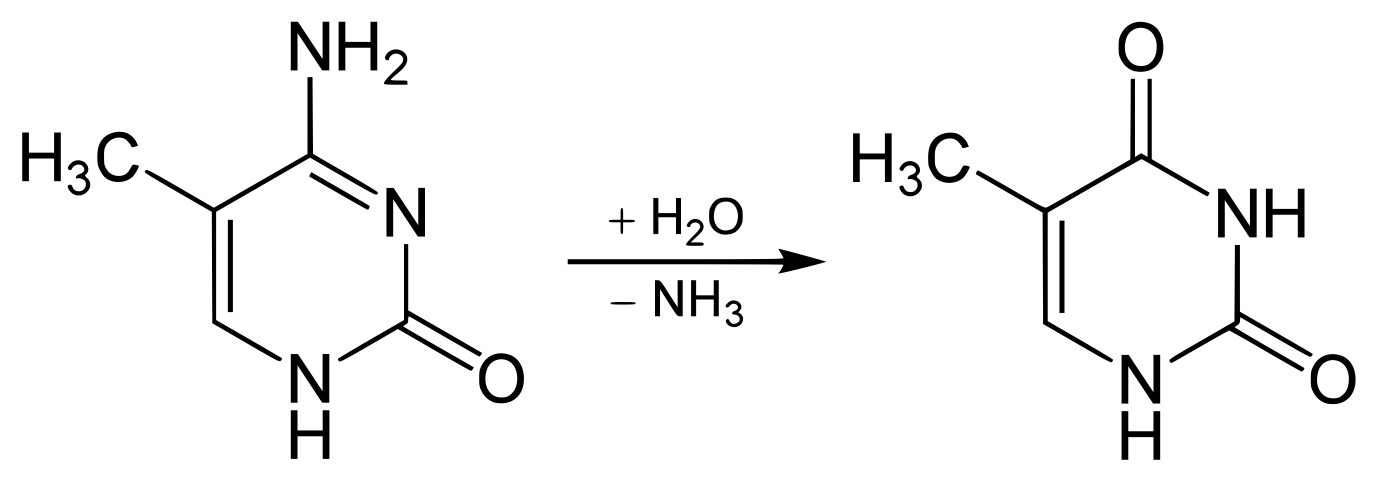
This is the most common single nucleotide mutation, even though most organisms have error checking mechanisms to detect and correct it. This results in a C to T transition on one strand, and a G to A transition on the other.
If D_S is the fraction of sites in an alignment that are transition differences, and D_V is the fraction of sites with transversions, then $$d = -\frac{1}{2}\ln(1 - 2D_S - D_V) - \frac{1}{4} \ln (1 - 2D_V). $$
As an example of these calculations, consider the following alignment of a small portion of the fibrinogen beta chain protein from humans (Homo sapiens), the baboon (Papio anubis) and the bottlenose dolphin (Tursiops truncatus).
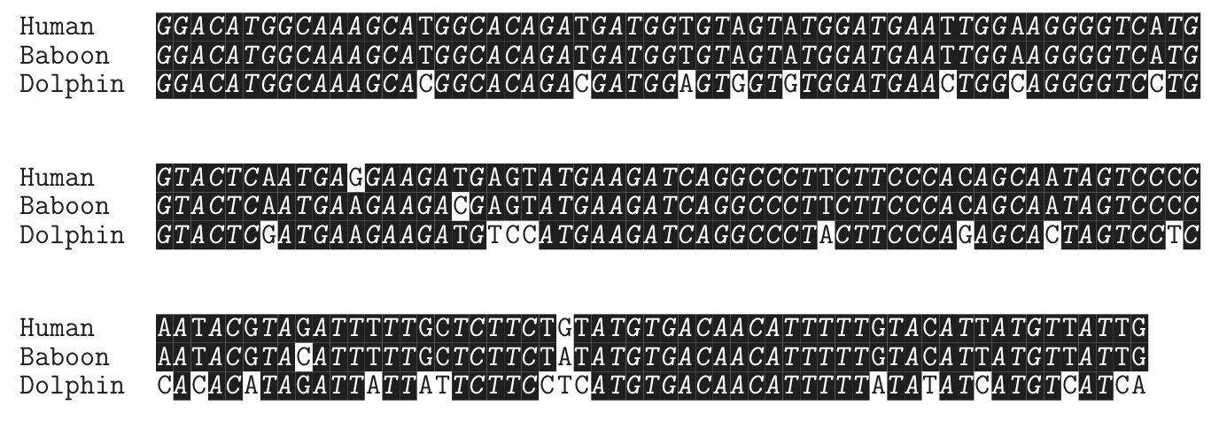
There are 177 sites in this alignment. Between the human and dolphin sequences there are 32 differences. Of the 32 differences, 21 are transitions, and 11 are transversions. Therefor D = \frac{32}{177} \approx 0.18, and the Jukes-Cantor distance is d_{JC} \approx 0.207. Under the Kimura model, D_S = \frac{21}{177} \approx 0.12, D_V = \frac{11}{177} \approx 0.06, and the distance is d_K \approx 0.211. It may seem surprising that the distances are almost the same under the two models, but this often happens when D is relatively small.
Between the human and baboon sequences there are only 4 differences, 3 transitions and 1 transversion. So D \approx 0.0226, and the Jukes-Cantor distance is d_{JC} \approx 0.023. For the Kimura model, D_S \approx 0.017, D_V = 0.0056, and d_K = \approx 0.023. Here again the change to the Kimura model does not significantly change the distance.
Under the models, distances should increase linearly in time. Using the Kimura model, this implies that since the ratio (human-to-dolphin distance)/(human-to-baboon distance) is \approx \frac{0.211}{0.023} \approx 9.2, the last common ancestor between humans and dolphins was about 9.2 as long ago as the last common ancestor between humans and baboons. From fossils and other evidence the best estimate of the human-baboon divergence is about 28 million years ago. Then the Kimura model would suggest that the human-dolphin divergence was about 260 million years ago. This is almost certainly too long ago to be correct. One major issue is that we are using a protein-coding sequence whose sites do not satisfy the assumptions of either the Jukes-Cantor or Kimura models.
Modelling site rate variation
All of the above models make the assumption that all sites behave identically and change at a constant rate. In some settings there are good assumptions, but often they are not. It is important to think about the particular data that is being analyzed.
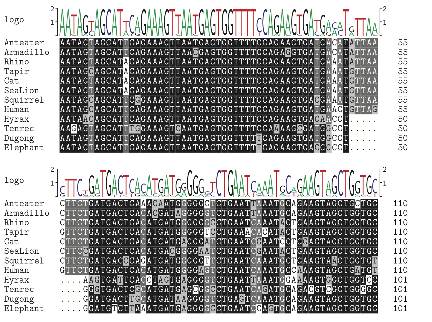
First let us consider variation between sites. Coding sequences (those that actually code for proteins) usually show much faster changes at the third codon site, because the genetic code is often redundant at that position. An example of this can be seen clearly in the BRCA1 (breast cancer susceptibility gene 1) alignment below (only a small fraction of each gene is shown here).
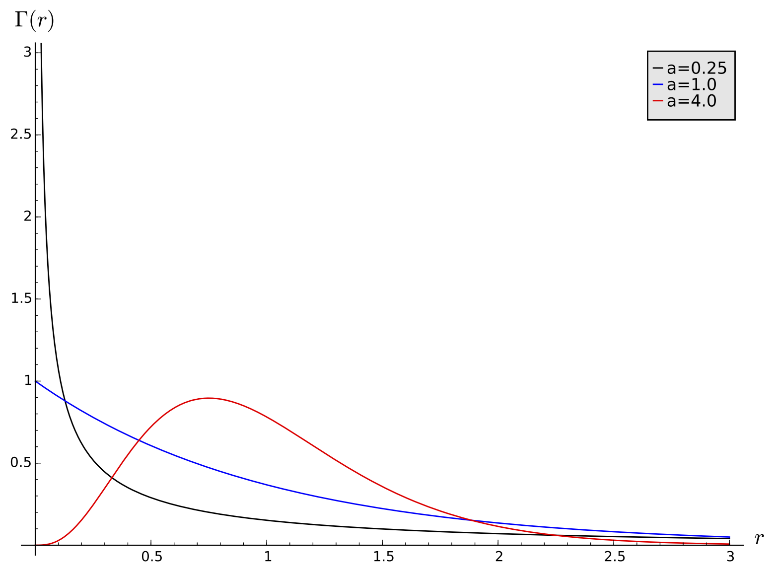
This can be handled in various ways. The data can be fit to models with a distribution of rates, often chosen to be the gamma distribution
where r is the rate of subsitution at a particular site relative to the average rate in the sequence as a whole and a is a parameter. The gamma function is defined by $$ \Gamma(a) = \int_{0}^{\infty} x^{a-1}e^{-x} \ dx. $$ The gamma distribution is used because with a single parameter it can model a variety of distributional patterns (cf. with the figure), and it has nice mathematical properties that let us exactly evaluate integrals that arise in its use.
The evolutionary distance for the Jukes-Cantor model with this distribution can be explicitly calculated as:
and then inverted to get
We can calculate the variance in a similar way to the Jukes-Cantor model:
Some sites might be under such strong selection pressure that they do not change at all. This can be modeled by introducing a fraction f of invariant sites - sites that do not change at all. It is possible to show that then $$ d = -\frac{3}{4} (1-f) \ln \left ( 1 - \frac{4 D}{3(1-f)} \right ). $$
General models
There are many generalizations of the Jukes-Cantor and Kimura models. One problem in both models is that the base frequencies are assumed to become uniform, whereas actual DNA often has an overall A+T or G+C bias. For example, the human genome has approximately 59% A and T bases, while the parasite Plasmodium falciparum has 83% A and T (!). A coding sequence might have different frequencies for all four bases. To account for this, we introduce a base probability distribution \pi = (\pi_A, \pi_G, \pi_C, \pi_T).
The Felsenstein model (sometimes referred to as 'F81' because of a different model introduced by Felsenstein in '84) generalizes the Jukes-Cantor model using the distribution \pi; the corresponding matrix is
although \alpha is now no longer interpretable as the rate of mutation (it is proportional to it).
The HKY model (Hasegawa, Kishino, and Yano, 1985) generalizes the Kimura model to non-uniform stationary distribution:
In the HKY model, the rate of all transitions (A \leftrightarrow G and C \leftrightarrow T) are equal. However, in many organisms these rates will be quite different. One important pathway for substitutions is the deamination of the methylated form of cytosine, which then changes to thymine. This reaction is so common that there are dedicated enzymes to correct it (G/T mismatch-specific thymine DNA glycosylase, TDG). The Tamura-Nei model (1993) allows for different rates for the two types of transitions:
These models are more complicated but even the Tamura-Nei model (often denoted as TN93) can be analyzed exactly. However, they still do not incorporate gaps.
The average overall substitution rate for the TN93 model is
and the corresponding evolution distance formula is
where
and S_1 is the proportion of site patterns with a T-C pair, S_2 is the proportion of A-G pairs, and V is the proportion of transversions.
A model is time-reversible if \pi_i q_{ij} = \pi_j q_{ji}. All the models above are time-reversible. It is not at all clear that requiring time-reversibility makes any biological sense, but in most cases it is a useful simplification. The reversibility condition is equivalent to the requirement that the matrix Q can be factored as $$Q = S \Pi $$ where \Pi is a diagonal matrix with the steady state frequencies \pi_i on the diagonal. The matrix S is symmetric, and its entries s_{ij} are sometimes called the exchangeabilities of i and j. The most general transition matrices that are actually used in applications is the time-reversible case, which has 12 free parameters.
Empirical protein models, entropy, and scoring matrices
Although they could in principle be modeled with methods similar to those used for DNA, in practice the evolution of protein sequences is handled more empirically. One reason for this is the large number of parameters that would need to be estimated; any errors in these estimations for an infinitesimal rate matrix would be amplified if a substantial amount of substitution takes place.
The first effort at modelling protein sequence evolution was led by Margaret Oakley Dayhoff, who began accumulating protein data, estimating transition rates, and implementing software in the 1960s. Some of these efforts resulted in the construction of the PAM family of protein scoring matrices. Before describing this family in detail, we first need some theoretical background on entropy and information theory and how they relate to scoring sequence alignments.
Entropy and information
The concepts in this section can be extended to continuous probability distributions, but we will only examine discrete ensembles here. Let the probability of x be p(x) = p_x (both notations can be convenient). We will consider sequences of characters from some alphabet A. The number of elements in the alphabet is N = |A|.
Note that since they are probabilities, we require \sum_{x \in A} p_x = 1 and 0 \le p_x \le 1.
Claude Shannon defined the information content of an outcome (sometimes called the surprisal) to be = \log_2(1/p_x). The use of the base-2 logarithm is not essential, but it is the most common choice.
The expected value of the information content is the entropy of the probability distribution. For a probability distribution P, this is often denoted by H(P):
When using base-2 logarithms, we say that there are H(P) bits of information per event for the distribution P. More rarely, sometimes the natural logarithm is used and then the units of entropy are called nats, or with base-10 logarithms the entropy is given in 'bans', or 'dits'. Unless indicated otherwise, we use base-2 logarithms for entropy and information-theoretic quantities. Some authors use the notation H_a(P) to denote an entropy using base a logarithms. Since \log_b(x) = \log_a(x)/\log_a(b), H_a(P) = \log_a(b) H_b(P), i.e. changing the base just multiplies all entropy values by the same constant.
The game of 20 Questions provides an example of thinking about entropy as information. If we played a strict form of the game in which only yes or no questions are allowed, and you are only allowed to have a 1-word answer, how many questions would we need to usually win? The answer is the entropy in bits of the distribution of answers chosen by some given pool of participants. If we play the game with small children, they tend to pick vertebrate animals (dogs, cats, lions, etc) rather frequently, and do not know too many words in general, so the entropy of their answers will be pretty low. At the other extreme, if we chose from the approximately 600,000 entries in the Oxford English Dictionary completely uniformly, each answer would have p = 1/600,000 probability and the entropy in bits would be
which means 20 yes/no (binary) questions should be just enough if we use optimal questions.
The entropy of the uniform distribution P, with p_i = \frac{1}{N}, is
This is the maximum possible entropy for a given set A.
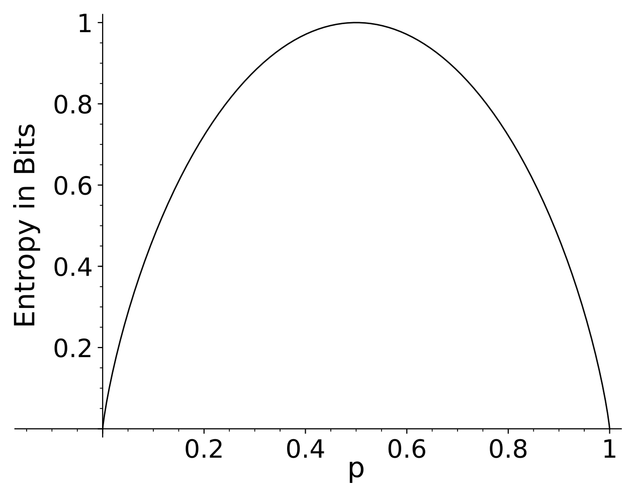
As another simple example, consider a random process that has 2 outcomes (one could imagine flipping a biased coin). The first outcome has probability p, and the second has probability 1-p. The entropy of a single event of this process is shown in the figure below for all p \in [0,1]. As this figure suggests, the limit \displaystyle \lim_{p\rightarrow 0} p \log(p) = 0, so if a probability of an outcome is 0 then we do not include it in the entropy.
The entropy of a joint distribution P(X,Y) is sometimes called the joint entropy, and is $$H(X,Y) = - \sum_{xy \in A_X A_Y} p(x,y) \log(p(x,y)) $$
If X and Y are independent random variables, then p(x,y) = p(x)p(y) and H(X,Y) = H(X) + H(Y):
This additive property for independent events is one of the major reasons for the definition of entropy.
Relative Entropy
The relative entropy of a distribution Q relative to another probability distribution P (with the same alphabet A) is: $$ H(Q||P) = \sum_{x \in A} q_x \log(\frac{q_x}{p_x}) $$ This is also known as the Kullback-Leibler "distance", but it is not symmetric, so it is better to call it the Kullback-Leibler divergence.
Using the elementary property of logarithms \log(a/b) = \log(a) - \log(b), we can also write the relative entropy as
The quantity C(Q,P) = - \sum_{x \in A} q_x \log(p_x) is called the cross-entropy, or sometimes the log-loss in machine learning contexts. From the above equality, we can write the cross-entropy in terms of an entropy and a relative entropy:
Gibbs' Inequality
The relative entropy is non-negative: H(Q||P) \ge 0. This is called Gibbs' Inequality. The easiest way to prove it is to use the convexity of the function \log(1/x). A function f(x) is convex on an interval (a,b) if for every x_1 and x_2 in (a,b), and every \lambda \in [0,1],
A function is strictly convex if the above inequality is an equality only for \lambda=0 and \lambda=1.
A very useful inequality for convex functions of random variables, Jensen's Inequality, is that the expected value E[f(x)] of f(x) is greater or equal to f(E[x]). If f is strictly convex, then equality is only possible if x is constant.
For the relative entropy, if we let f(x) = \log(1/x), Jensen's inequality gives us
and since \log(1/x) is strictly convex, the relative entropy is only zero if P=Q.
If P is the uniform distribution p_i = \frac{1}{N}, then H(Q||P) = H(P) - H(Q) (proving this is a good exercise!).
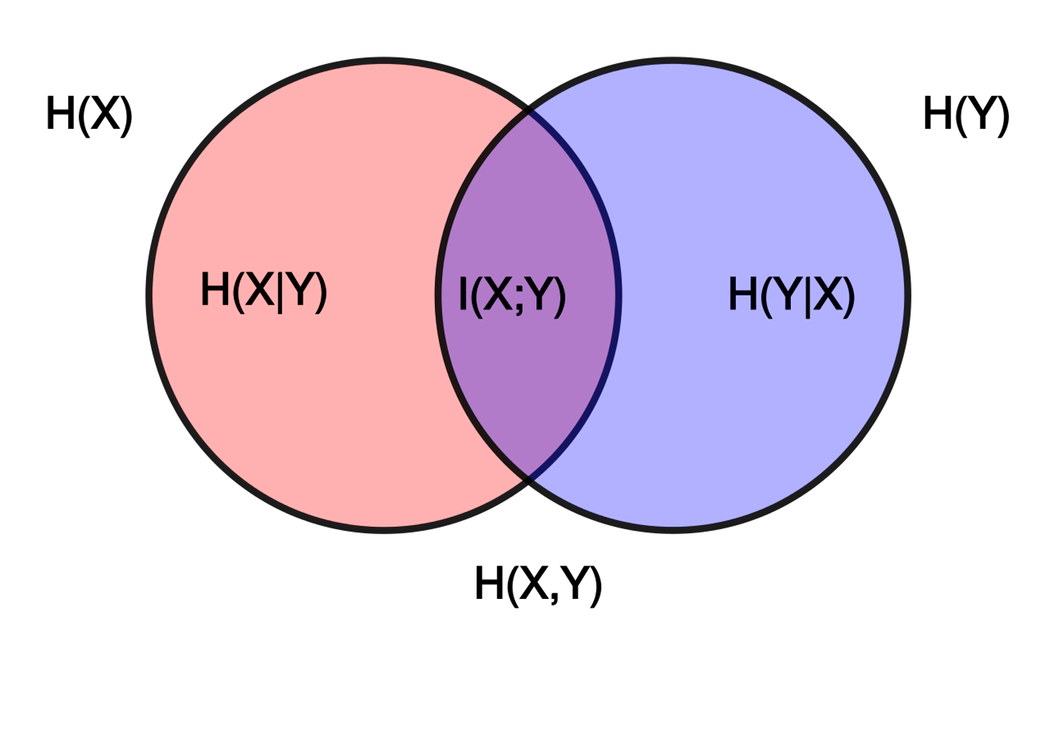
Conditional Entropy and Mutual Information
If we are interested in a distribution X conditioned on a distribution Y, then we can denote the conditional entropy as H(X | Y). This is $$H(X | Y) = \sum_{y \in A_Y} p(y) \left[ \sum_{x \in A_X} p(x | y) \log \frac{1}{p(x | y)} \right] = \sum_{x,y \in A_X,A_Y} p(x,y) \log \frac{1}{p(x | y)} $$
For example, suppose Y is obtained by flipping a coin. If the coin comes up tails (T), then we let x=1. If it comes up heads (H), we roll a six-sided die to determine x. The joint probability distribution is p(T,1) = 1/2 and $$p(H,1) = p(H,2) =p(H,3) =p(H,4) =p(H,5) =p(H,6) = 1/12. $$ The conditional entropy H(X|Y) is 1/2(\log(1)) + 6/12 \log(6) = \log(6)/2.
For a joint probability distribution, the joint entropy can be decomposed as follows (sometimes this is called the 'chain rule' for joint entropy):
We define the mutual information between X and Y as
This can also be computed as
I.e. the mutual information is the relative entropy of the joint distribution of X and Y compared to the product distribution. Very often the term relative entropy is used in this context, and it may be more helpful to think of it as the mutual information. Mutual information appears in various contexts in bioinformatics.
We can get a little more baroque and decompose the conditional mutual information between X and Y, given Z:
Exercise
The Kullback-Leibler divergence is not a distance on a space of probability distributions, but there is a distance which has some related properties. If we have two probability distributions P and Q on the same discrete set X, then define the distance to be:
This is similar to the Bhattacharyya distance
Show that infinitesimally d_M is close to the relative entropy H(P||Q) by computing the first few terms of the power series of each quantity in t for Q = P + tF where \sum_X F = 0.
Choice of model and alphabet
The choice of alphabet is important in considering entropy. For example, consider a sequence of symbols
ABABABABABABABAB\ldots
emitted by some probabilistic process. If we consider each letter individually, the proportions of the letters are p_A = p_B = 0.5, with an entropy of 1 bit. But if we consider pairs of letters, then p_{AB} = 1 and p_{AA} = p_{BB} = p_{BA} = 0, which has an entropy of 0.
If we wish to understand the complexity of a process, sometimes a simple notion of entropy fails to measure what we want. Besides the choice of alphabet, there are other modeling choices we must make about the process under observation. Perhaps the most general notion of complexity for a sequence is the Kolmogorov complexity, which is defined (loosely) as the length of the shortest computer program that could generate that output.
Splice site example
An example may help illustrate some of the concepts in this section. In the process of transcription from DNA to RNA, genes are often spliced. The removed sequences are called introns, and the remaining spliced together pieces are called exons. In order for the splicing enzyme complexes to recognize the correct locations to cut and splice, there must some information in the sequence. We can use information theory to try to characterize this. We will focus on the 3' end of the intron; a similar analysis could be done for the 5' end. The 3' end of an intron involved in splicing is called the acceptor site. (Recall that DNA strands have a direction, and genes are read in the 5' to 3' direction.)
It is known that most acceptor sites in eukaryotes end with the nucleotide sequence AG. We selected approximately 10,000 introns from the human genome to analyze. For our acceptor site analysis we took 30 bases on the intron side of the splice and 20 bases on the exon side.
Here are 20 of these sequences chosen at randomly. The space in each sequence is the location of the splice.
tcacctctctggttcctctcgccctttcag gtggggacccatcgtgaaga
ttaaagtataattcttgtacttcaataaag gcagcagctttagcatctct
tgacatcataattttacatacaatttatag gaatgtccagaaagagaagt
cttatccttcccattgtttttttctgccag atgagagatgttcagttcaa
cacctcctcacgcagccccttcccccacag ggccggctcccaggcctcag
tgtttatgcctgtattattttaacctgtag aatcttaagaagattcaaga
attgttatgtacatgtttttccacttttag cctttggagactcgacttat
gcactgacttcctgggtctctgtcttccag aacatccaccagtggtgtgg
tagtctgtatctcttttctttcttcccaag agtcatctggggaacgtgtt
ttccctttacttcttgattattttttcaag gtctatgtacagacatggag
acccatattcctccttcccttactttccag gcccatcccgtggcggttgc
cttcctcacggggccgcaattcgctttcag tacacggaaggagacggcga
cactgtattttaattctttttctcctgtag gaaaaagaagaactgattga
gtctgtgtttattgtgtcttatttccctag ctccagtggctgttggacaa
atcttagtaagtttgctattttattttcag ggccgaattacaaaagtatt
ttttgttatatttggtgtttttaataatag gtttcagaagatgatttctc
ccagtaatttattccatgtttgcatttcag cttgtgcgatctgcctcatt
aattcttaataatccctgcattactcttag gtaaatattgcaacttcagc
gcaaatgaccactttcaaaccgttttccag aatgataatggtgacagcta
acctccacctgtgctgtctctttcctgcag caacacgggattcccatccc
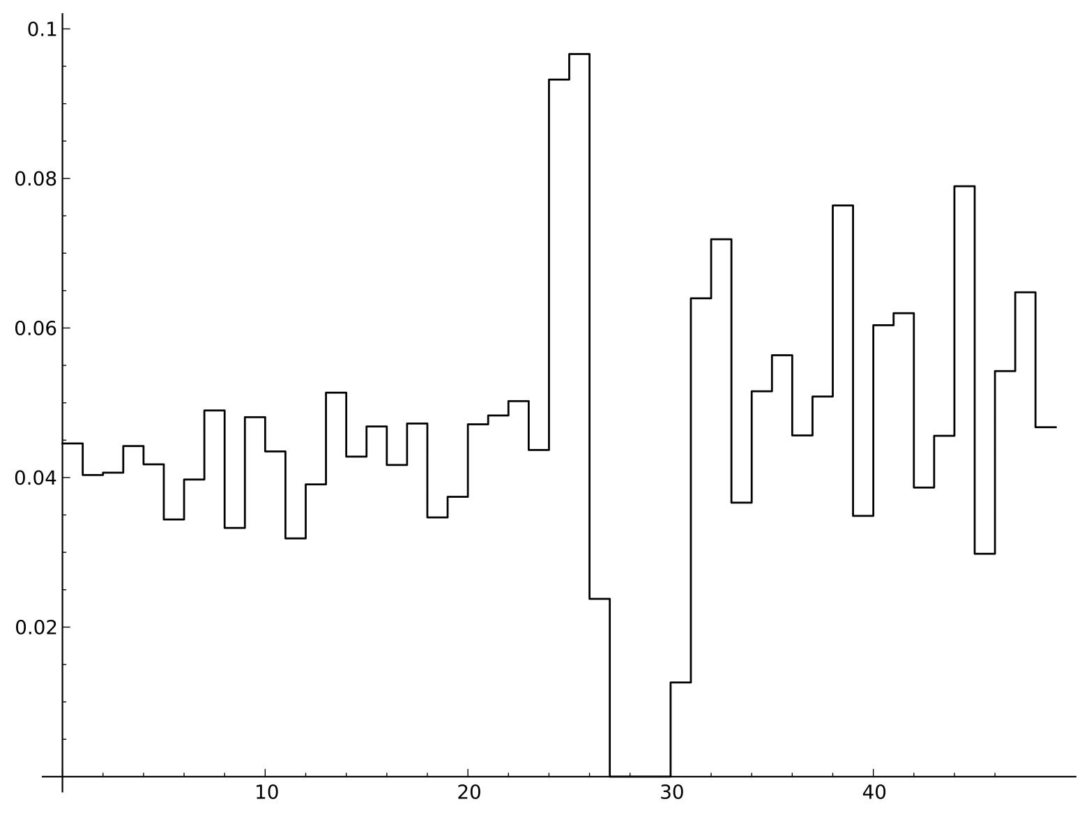
For each of the 50 sites in the sequences we can compute the relative entropy of the site nucleotide frequencies with the overall frequencies. In this set of data, the overall frequencies of the nucleotides was p_A = 0.224, p_C=0.243, p_G=0.199, p_T=0.334.
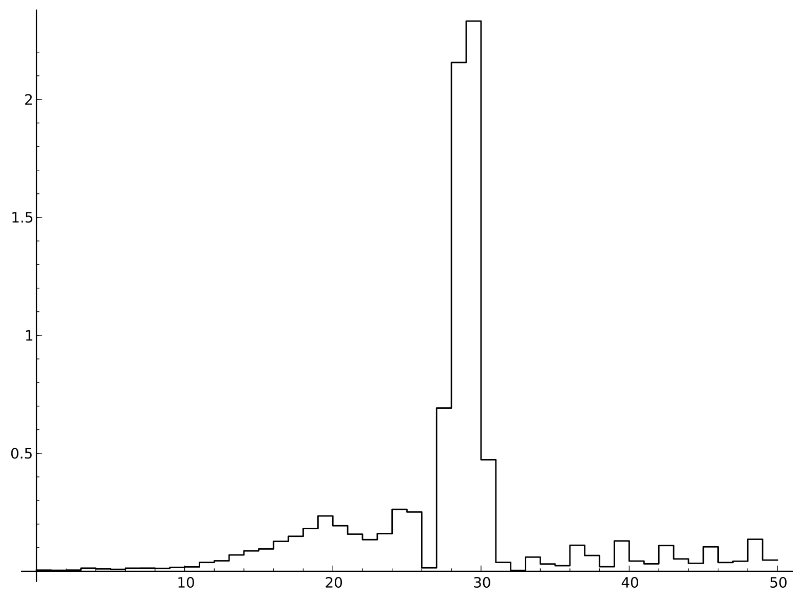
Relative entropy of sites near splice junctions
There are a number of interesting features in the relative entropy plot. The large spike is the AG present in all the sequences. Because A is more common than G in the overall frequencies, the invariant A site does not have quite as large a relative entropy as the G. After the splice, we can see a possible influence of the structure of the genetic code in the coding region, as the relative entropy seems to vary periodically every three bases. Upstream of the splice we see that there is a substantial deviation from the background frequency in an approximately 15-base window. Somewhat surprisingly, the identity of the site two bases upstream of the AG splice site appears to be completely irrelevant.
A convenient way to visualize the sequence content using relative entropy is the sequence logo. In the logo, the total height alloted to each site is proportional to the relative entropy of that site. Within that alloted total height, the fraction used for each letter is the frequency of that letter at that site. The sequence logo makes it clear that there is a CT (pyrimidine) rich region upstream of the splice site.
![]()
Sequence logo (relative to uniform distribution) of sites near splice junctions
The preceding analysis only considers each site independently. To explore possible correlations between neighboring sites, we can compute the mutual information between each pair of neighbors:
Mutual information of sites near splice junctions
It may be somewhat counter-intuitive that the invariant AG pair has a mutual information of 0, but since there is no variation at those sites the entropy of the joint distribution is 0. More interestingly, the highest values of the mutual information are five and six bases upstream of the splice site, at the end of the pyrimidine rich region. This comes from an enrichment of TT or CC pairs compared to what would be expected from the product of the individual site frequencies.
Scoring Matrices
This section will mostly be phrased in terms of protein sequences, because that is its most important application. The same theory can also be applied to nucleotide or other sequences (codon-based models, for example). Because the twenty standard amino acids have very different chemical and physical properties (such as charge and size), different amino acid substitions will have very different effects. Large changes to the protein will result in a lack of function, and for essential proteins such changes would often be lethal. Protein scoring matrices try to quantify this, usually from observed changes. As an example, consider the alignment of hemoglobin subunit alpha proteins shown below:
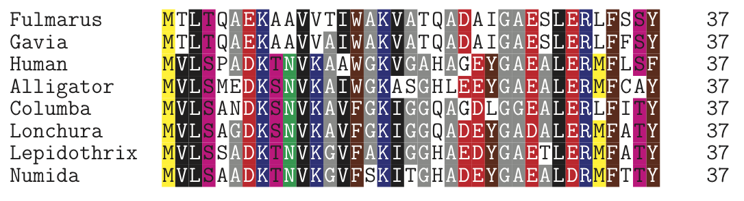
The colors in this alignment have been chosen to reflect chemical properties. We can see that the changes within each site are not uniform. For example, there are several columns with only the negatively charged D (aspartic acid) or E (glutamic acid) amino acids.
We assume we have a model for the probability of a change in amino acids in a protein sequence, where each site behaves identically and independently. More precisely, we have a transition matrix q_{i,j} giving the probability of amino acid i changing to amino acid j. We also have a background distribution of individual amino acids, p_i, which is usually estimated as the proportion of amino acid i in a proteomic database for a particular organism or collection of organisms. Then we can form a log-odds scoring matrix:
$$S_{i,j} = \log(\dfrac{q_{i,j}}{p_i p_j})/\lambda $$ where \lambda is an arbitrary scaling parameter.
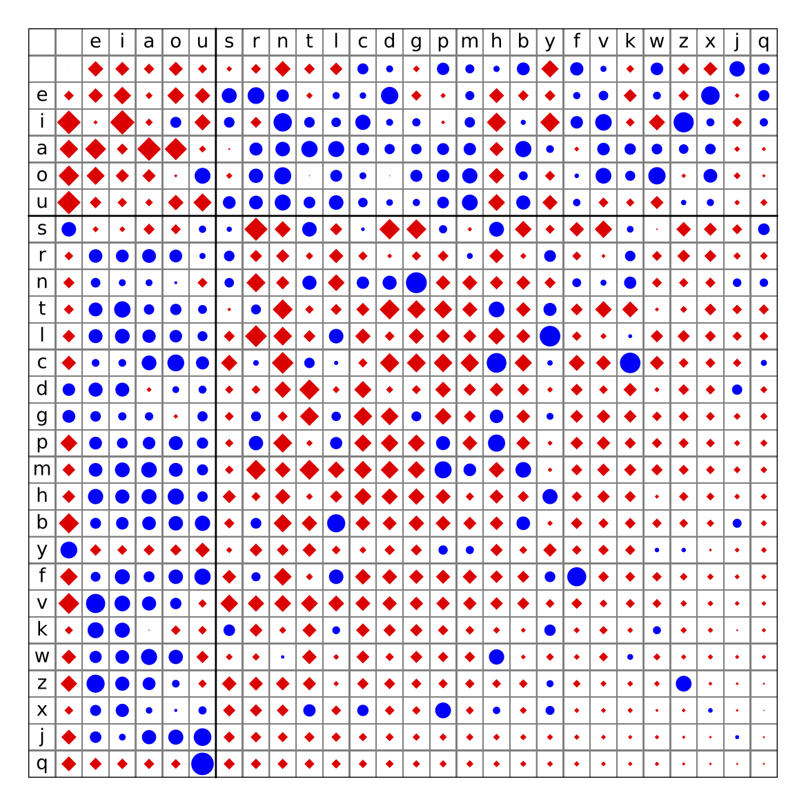
Such log-odds scores are a good way to quantify the difference between two distributions. Here is a simple non-biological example, using the words of the English language as data. We can compute the frequencies of each letter, p(i), and then compare them to the conditional probability of seeing one letter after another, p(i|j). This is equivalent to comparing the joint distribution q(i,j) to the product distribution p(i)p(j). Counting a whitespace as a extra letter, the log of the ratios are visualized below, with red diamonds for negative log-odds (under-represented pairs of letters), and blue for positive log-odds (over-represented pairs).
When using log-odds scores for sequence alignments, the expected score for each site in an alignment between random sequences is \sum p_i p_j S_{ij}.
The relative entropy of the distribution q_{i,j} compared to a product distribution p_i p_j, often just referred to as the entropy of the scoring matrix, is \sum q_{ij} S_{ij}. This can be interpreted as the expected score of each site in an alignment between two related sequence whose divergence is consistent with the transition matrix q.
PAM and BLOSUM
The historically first important protein scoring matrix family, the PAM family, was developed by Margaret Dayhoff's lab, starting in the late 1960s. PAM initially stood for "point accepted mutation". This refers to the assumptions that amino acid changes occur at each site independently, and that if very similar (over 85% identical) protein sequences are compared it is reasonable to assume that each differing site has only changed once.
The idea used in PAM is to first construct a matrix M reflecting the probabilities of amino acid changes over short time scales, and then extrapolate these changes. The advantage of this method is that the short time scale matrix is derived from very similar protein sequences, in which the alignments are largely unambiguous. A disadvantage is that any errors in the initial matrix will be hugely amplified by the extrapolation process.
Suppose we use N total amino acids in the protein sequence alignments, the number of amino acid i is n_i, and that the proportion of amino acid i is p_i. We count the observed changes between amino acids in a matrix A. Then an off-diagonal entry of the transition matrix M is given by $$M_{i,j} = \frac{\lambda A_{i,j}}{N p_j} $$ which gives the rate of change of amino acid j to amino acid i. The parameter \lambda is used to rescale the rates of change so that after one transition, a protein sequence would remain 99% identical.
Diagonal entries of M are given by $$M_{i,i} = 1 - \lambda m_i $$ where m_i is the mutability of amino acid i:
The scoring matrix derived from M is the PAM1 matrix; by design it should be optimal for sequences that are 99% identical. We can extrapolate to more divergent sequences by using powers of M; the scoring matrix derived from the nth power of M is denoted PAMn. In practice, the most divergent PAM matrix used is PAM250.
The actual scoring matrix entries are given by
Although it is not immediately obvious, the PAM matrices are symmetric.
Dayhoff's PAM matrices were based on a rather limited set of protein alignments. Her work method has been used several times since then with larger databases. One of the improved matrix families is known as JTT (initials of the authors Jones, Taylor, and Thornton).
The most commonly used protein scoring matrix family, the BLOSUM family, tries to avoid the extrapolation step by deriving the transition rates of amino acid directly from more divergent protein alignments. This method should be superior but there is a dangerous circularity present, since a scoring matrix must be used to generate the alignments. The creators of the BLOSUM family (Henikoff and Henikoff) got around this circularity by iterating their procedure several times.
In the BLOSUM family, the percentage of sequence identity used in the alignments blocks is used in the matrix name. Thus BLOSUM45 is derived from blocks of protein alignments that are 45% identical. It is comparable to the PAM250 matrix; they each have a relative entropy of approximately 0.4 bits. The BLOSUM80 matrix is comparable to the PAM120 matrix; their relative entropy is about 1.0 bit.
Implied log-odds matrices
The PAM matrix is not derived directly from a log-odds construction. Many other scoring matrices have been proposed for protein and DNA sequences which are also not derived in the log-odds framework. Nevertheless, they usually can be interpreted as if they were.
Suppose we are given a scoring matrix S. We can intrepret the entries of this matrix as scaled log-odds scores:
$$S_{i,j} = \frac{1}{\lambda} \log{\frac{Q_{i,j}}{P_i \tilde{P}_j}} $$ if we can find a consistent choice of transition frequencies Q and \lambda with P_i = \sum_j Q_{i,j} and \tilde{P}_j = \sum_i Q_{i,j}. For most reasonable scoring matrices this is possible.
In the special case where we know in advance the distributions P and \tilde{P}, it is relatively simple to show there is a unique Q and \lambda if the expected random score \sum_{i,j} S_{i,j} P_i \tilde{P}_j is negative and there is at least one positive score. We will briefly sketch the argument. More detail can be found in several papers of Stephen Altschul and Samuel Karlin, among others, who were the primary developers of this theory from about 1990 - 2010.
Since Q is a probability distribution, \sum_{i,j} Q_{i,j} - 1 = 0. Writing this in terms of S, we define the function
We want to show there is a unique positive root g(\lambda) = 0.
Note that g(0) = 0, and
Since we are assuming that \sum_{i,j} S_{ij} P_i \tilde{P}_j < 0, g'(0) < 0. Taking another derivative we find that
Now the assumption that some S_{i,j}>0 means that $$\lim_{\lambda \rightarrow \infty} g = \infty $$
and there is a unique root.
Example: The standard scoring system for DNA used by the BLAST suite of programs gives a score of 1 for any match, and -2 for any mismatch. We will calculate the implied probabilities of this scoring matrix. Since all letters are treated the same, we know that the background probabilities are P_i = 0.25 for each letter i.
Then in the sum \sum Q_{i,j} = 1, we can substitute using the relation \lambda S_{i,j} = \log_2(\frac{Q_{i,j}}{P_i P_j}), or Q_{i,j} = P_i P_j 2^{\lambda S_{i,j}} to get
and with our particular numbers, and with x = 2^{\lambda},
so x^3 - 4x^2 + 3 = 0 which has positive roots x = 1 and x \approx 3.79128784747792. We want a strictly positive \lambda = \log_2(x), so we use the larger root.
Plugging in this value of x or \lambda into the Q equation we find Q_{i,i} = x/16 = \approx 0.23695549046737 and Q_{i,j} = x^{-2}/16 \approx = 0.00434816984421.
Under this model, we are assuming a level of divergence between related sequences of D = 4 Q_{i,i} \approx 0.947822, or almost 95\% sequence identity. When aligning less similar DNA sequences, it may be advantageous to use a scoring matrix whose underlying model better matches that level of similarity.
Does it matter
If you are aligning very similar proteins (more than 90% identical), it probably won't make much of a difference what protein scoring matrix you use. But for more distant homologs the scoring matrix can make a big difference, and so can the alignment program you use.
The following alignments are between the human and yeast (Saccharomyces cerevisiae) hexokinase protein, using NCBI's blastp. The first alignment uses the scoring matrix BLOSUM45; the second alignment used the PAM30 matrix. The PAM30 matrix is optimized for very similar proteins, while BLOSUM45 is optimized for only 45% sequence identity. Because of this, the BLOSUM45 alignment is longer and probably better by most criteria.
Range 1: 5 to 479

Alignment statistics for match #1 Score Expect  Identities  Positives   Gaps
221 bits(742)   3e-69   164/488(34%)    270/488(55%)    31/488(6%)

Query  448  GSGKGAAMVTAVAYRLAEQHRQIEETLAHFHLTKDMLLEVKKRMRAEMELGLRKQTHNNA  507
            G  K  A   ++A    E   +I +    F +  + L +V K    E+  GL K+  N
Sbjct  5    GPKKPQARKGSMADVPKELMDEIHQLEDMFTVDSETLRKVVKHFIDELNKGLTKKGGN--  62

Query  508  VVKMLPSFVRRTPDGTENGDFLALDLGGTNFRVLLVKIRSGKKRTVEMHNKIYAIPIEIM  567
             + M+P +V   P G E+G++LA+DLGGTN+RV+LVK+      T +     Y +P ++
Sbjct  63   -IPMIPGWVMEFPTGKESGNYLAIDLGGTNLRVVLVKLSGN--HTFDTTQSKYKLPHDMR  119

Query  568  QGTG-EELFDHIVSCISDFLDYMGIKGPR--MPLGFTFSFPCQQTSLDAGILITWTKGFK  624
                 EEL+  I   + DF+    +   +  +PLGFTFS+P  Q  ++ GIL  WTKGF
Sbjct  120  TTKHQEELWSFIADSLKDFMVEQELLNTKDTLPLGFTFSYPASQNKINEGILQRWTKGFD  179

Query  625  ATDCVGHDVVTLLRDAIKRREEFDLDVVAVVNDTVGTMMTCAYEEPTCEVGLIVGTGSNA  684
              +  GHDVV LL++ I +RE + +++VA++NDTVGT++   Y +P  ++G+I GTG N
Sbjct  180  IPNVEGHDVVPLLQNEISKRE-LPIEIVALINDTVGTLIASYYTDPETKMGVIFGTGVNG  238

Query  685  CYMEEMKNVEMVEGD-------QGQMCINMEWGAFGDNGCLDDIRTHYDRLVDEYSLNAG  737
             + + + ++E +EG           M IN E+G+F DN  L   RT YD  VDE S   G
Sbjct  239  AFYDVVSDIEKLEGKLADDIPSNSPMAINCEYGSF-DNEHLVLPRTKYDVAVDEQSPRPG  297

Query  738  KQRYEKMISGMYLGEIVRNILIDFTKKGFLFRGQISETLKTRGIFETKFLSQIESDRLAL  797
            +Q +EKM SG YLGE++R +L+++ +KG++++ Q    LK   I +T + ++IE D +
Sbjct  298  QQAFEKMTSGYYLGELLRLVLLELNEKGLMLKDQDLSKLKQPYIMDTSYPARIEDDPFEN  357

Query  798  LQ-VRAILQQ-LGLNSTCDDSILVKTVCGVVSRRAAQLCGAGMAAVVDKIRENRGLDRLN  855
            L+    I+Q+ +G+ +T  +  L++ +C ++  RAA+L   G+AA+  K     G
Sbjct  358  LEDTDDIFQKDFGVKTTLPERKLIRRLCELIGTRAARLAVCGIAAICQKRGYKTG-----  412

Query  856  VTVGVDGTLYKLHPHFSRIMHQTVKEL------SPKCNVSFLLSEDGSGKGAALITAVGV  909
              +  DG++Y  +P F     + ++++      + K  ++ + +EDGSG GAA+I A+
Sbjct  413  -HIAADGSVYNKYPGFKEAAAKGLRDIYGWTGDASKDPITIVPAEDGSGAGAAVIAALSE  471

Query  910  RLRTEASS  917
            +   E  S
Sbjct  472  KRIAEGKS  479

Range 1: 74 to 307

Alignment statistics for match #1 Score Expect  Method  Identities  Positives   Gaps
129 bits(297)   4e-34   Composition-based stats.    108/261(41%)    128/261(49%)    60/261(22%)

Query  520  PDGTENGDFLALDLGGTNFRVLLVKIRSGKKRTVEMH------NKIYAIPIEIM-----Q  568
            P G E G++LA DLGGTN RV LVK  SG       H       K Y  P + M     Q
Sbjct  74   PTGKESGNYLAIDLGGTNLRVVLVKL-SGN------HTFDTTQSK-YKLPHD-MRTTKHQ  124

Query  569  GTGEEL--FDHIVSCISDFL-DYM------GIKGPRMPLGFTFSFPCQQTSLDAGILITW  619
               EEL  F      I D L D+M        K   +PLGFTFS+P  Q   + GIL  W
Sbjct  125  ---EELWSF------IADSLKDFMVEQELLNTKDT-LPLGFTFSYPASQNKINEGILQRW  174

Query  620  TKGFKATDCVGHDVVTLLRDAIKRREEFDL--DVVAVVNDTVGTMMTCAYEEPTCE--VG  675
            TKGF   +  GHDVV LL + I  RE   L  ++VA +NDTVGT+    Y +P  E   G
Sbjct  175  TKGFDIPNVEGHDVVPLLQNEISKRE---LPIEIVALINDTVGTLIASYYTDP--ETKMG  229

Query  676  LIVGTGSNACYMEEMKNVEMVEG---DQ----GQMCINMEWGAFGDNGCLDDI--RTHYD  726
             I GTG N  + +   ++E  EG   D       M IN E G F DN  L  +  RT YD
Sbjct  230  VIFGTGVNGAFYDVVSDIEKLEGKLADDIPSNSPMAINCEYGSF-DNEHL--VLPRTKYD  286

Query  727  RLVDEYSLNAGKQRYEKMISG  747
              VDE S   G Q +EKM SG
Sbjct  287  VAVDEQSPRPGQQAFEKMTSG  307
Synonymous and Nonsynonymous Substitutions
Because of the redundancy in the genetic code, in a protein coding sequence a change in a single nucleotide can have no effect on the translated product. In this case we say the substitution is synonymous. If instead the change does cause a change in the amino acid sequence of the translated sequence, then it is a nonsynonymous change.
For highly conserved protein domains we expect that the rate of synonymous substitutions would usually be much larger than nonsynonymous substitutions. However in some proteins, such as those involved in the immune system, the protein sequence may be under diversifying selection, and nonsynonymous substitutions would be more common. Therefore it is an important problem to be able to quantify these rates.
There are many different methods for precisely quantifying the synonymous and nonsynonymous substitution rates. We will only describe the simplest such method, similar to that of Nei and Gojobori's 1986 paper, illustrated by a small example:
 M   P   Q   S   T   R   L
ATG CCT CAA TCT ACA CGG CTT

ATG CCC CAT AGT ACA TGC CTT
 M   P   H   S   T   C   L
The first step is to calculate the number of possible synonymous and nonsynonymous changes for the pair of sequences. We will denote these by L_s and L_n. The sum of these will be the length L of the alignment; in our example L=21, so L_s + L_n = 21. Thus we only need to calculate L_s.
Each nucleotide letter in each sequence can be changed to three others; the fraction of these three that are synonymous will be counted as part of L_s, with the results averaged over both sequences. In the first codon in our example, the top sequence is ATG. Since ATG is the only codon that codes for methionine (M), any change in any of three letters is nonsynonymous, and we count nothing towards L_s.
For the second codon, the top sequence has CCT. The first and second letters must be C to code for proline, but the third letter can be anything. Thus the third site in the codon counts for 3/3 = 1 for L_s. The same is true for the CCC codon in the second sequence, so the average is (1+1)/2 = 1.
In the third codon, again only the third codon can be changed, but for CAA the only possibility is CAG, and for CAT the only synonymous change is to CAC. Thus each sequence has 1/3 contribution to the average.
The fourth codon is perhaps a bit counterintuitive, since the two sequences both code for serine (S), but with widely separated triplets. The TCT triplet can be changed in its third site, contributing 3/3. The AGT triplet can only tolerate a change to AGC (we only considering single-letter changes), contributing 1/3. Their average contribution is (1+3)/6 = 2/3.
The fifth codon has two copies of ACA, coding for threonine (T). Again the third letter can be anything, so this codon contributes 1 to L_s.
For the sixth codon the CGG (R) has four synonymous possible changes, while the TGC (C) has only one, contributing (4+1)/6 = 5/6. The seventh codon contributes 1, just as the fifth.
In total L_s = 0 + 1 + 1/3 + 2/3 + 1 + 5/6 +1 = 29/6, so L_n = 21 - 29/6 = 97/6.
The second step is to count how many synonymous and nonsynonymous changes appear. In some cases this is ambiguous, when there is more than one change within a codon. We will adopt the simple procedure of averaging uniformly over all the possible paths of single-nucleotide changes.
In our example, there are no changes in codons 1, 5, and 7. There is an unambiguous synonymous change in codon 2, and an unambiguous nonsynonymous change in codon 3. For codon 4, two paths of changes are possible:
or
both of which involve 2 nonsynonymous changes.
Codon 6 also has two paths:
or $$\text{CGG} \rightarrow \text{TGG} \rightarrow \text{TGC}. $$
The first path has a synonymous change followed by a nonsynonymous change, while the second has two nonsynonymous changes. We use the average of these, counting the codon's changes as 1/2 synonymous and 3/2 nonsynonymous.
The proportion of synonymous changes is then D_S = \frac{1 + 1/2}{29/6} = \frac{9}{29}, and the proportion of nonsynonymous changes is D_N = \frac{1 + 2 + 3/2}{97/6} = \frac{27}{97}. If these are not very small, as is the case in our toy example, it may make sense to correct them with a model such as the Jukes-Cantor + Gamma rate variation described earlier. For D_S and D_N less than about 0.05, such a correction may not improve the accuracy of the ratio by a meaningful amount.
In our example, if we use the uncorrected values we find \frac{D_N}{D_S} = \frac{87}{97}, which is close to 1, suggesting that this sequence is not under either extremely strong purifying or positive selection.
A major problem in applying this idea in practice is choosing the length of sequences to compare. An overly large window will mix together regions of a protein that are under very different selection pressures, while too small a window will introduce too much variation to make robust statistical inference possible.
Another issue with these computations is the interplay between the transition/transversion ratio and the structure of the genetic code. Transitions are usually much more frequent than transversions, but they also result in synonymous changes when occuring in the third codon position. This makes the ratio \frac{D_N}{D_S} smaller even if there is not purifying selection at work.
Exercise: Calculate the synonymous and non-synonymous rates of substitution between the two sequences below.
 G   H   I   G   T   W
GGA CAC ATT GGC ACA TGG

GGA CAT ATC AGT ACA TCC
 G   H   I   S   T   S